China

Analysis on Turkey is available below. Highlights A dovish Fed or robust U.S. growth does not constitute sufficient conditions for a bull market in EM. China’s business and credit cycles are much more important factors for EM than those of the U.S. A recovery in the Chinese economy and global manufacturing is not imminent. The common signal reverberating from various financial markets is that the risks to the global business cycle are still skewed to the downside. Feature Current investor perceptions of emerging markets are mixed. Some expect EM to benefit greatly from low U.S. interest rates. These investors view even a partial trade deal between the U.S. and China as sufficient for EM to embark on a bull market. BCA’s Emerging Markets Strategy team disagrees with this narrative. We deliberated the significance of the U.S.-China confrontation to EM in our September 19 report; therefore, we will not go over this subject here. Rather, in this report we discuss some of the more common misconceptions surrounding EM currently, and infer what these mean for investment strategies. Perception 1: The share of resource sectors (materials and energy) in the EM equity benchmark has declined substantially. This along with the expanded role of consumers and consumer stocks (Alibaba, Tencent and Baidu) in EM economies and equity markets has made their share prices less exposed to the global trade cycle and commodities prices. Reality: It is true that in many EM bourses, the weight of consumer stocks has been growing. Nevertheless, their financial markets in general, and equity markets in particular, remain very sensitive to the global trade cycle and commodities prices. Chart I-1 illustrates that the aggregate EM equity index has historically been and continues to be strongly correlated with the global basic materials stock index. The latter includes mining, steel and chemical companies. Global materials stocks also exhibit a very strong correlation with Chinese banks’ share prices. Moreover, global materials stocks also exhibit a very strong correlation with Chinese banks’ share prices (Chart I-2). The rationale for the high correlation is that both mainland banks’ profits and global demand for basic materials are driven by a common factor: China’s business cycle. Chart I-1EM And Global Materials Stocks Move Together EM And Global Materials Stocks Move Together EM And Global Materials Stocks Move Together Chart I-2Chinese Bank And Global Materials Share Prices Are Highly Correlated Chinese Bank And Global Materials Share Prices Are Highly Correlated Chinese Bank And Global Materials Share Prices Are Highly Correlated For example, construction in China is contracting (Chart I-3), which entails both higher NPLs for Chinese banks and lower demand for basic materials. China accounts for about 50% of global consumption of industrial metals, cement and many other basic materials. Finally, EM ex-China bank stocks also correlate strongly with global basic materials share prices. The basis is as follows: Many emerging economies export raw materials, and commodities price fluctuations impact their business cycle, exports and exchange rates. Chart I-3China: Construction Activity Is Contracting China: Construction Activity Is Contracting China: Construction Activity Is Contracting Chart I-4High-Yielding EM: Currencies And Local Bond Yields High-Yielding EM: Currencies And Local Bond Yields High-Yielding EM: Currencies And Local Bond Yields Historically, in high-yielding EM markets, currency depreciation has led to higher interest rates and lower bank share prices, and vice versa (Chart I-4). Lately, EM bond yields have not risen in response to EM currency depreciation. However, we believe this correlation will soon be re-established if EM currencies continue drifting lower.  In short, China’s money/credit cycles drive not only the mainland’s business cycle, banking profits and NPLs, but also global trade and commodities prices. The latter two - via their impact on exchange rates and in turn interest rates - have historically explained credit and domestic demand cycles in high-yielding EM. Perception 2:  EM stocks are a high-beta play on the S&P 500, i.e., EM equities outperform when the S&P 500 rallies, and vice versa. Reality: Since 2012, the beta for EM equity versus the S&P 500 has often been below one (Chart I-5). Furthermore, since 2012, EM share prices often failed to outpace their DM peers during global equity rallies. Indeed, EM relative equity performance versus DM, as well as the EM ex-China currency total return index, have been closely tracking the relative performance of global cyclicals versus global defensive stocks (Chart I-6). Chart I-5EM Equities Beta To The S&P 500 EM Equities Beta To The S&P 500 EM Equities Beta To The S&P 500 Chart I-6Global Cyclicals-To-Defensives Equity Ratio And EM Global Cyclicals-To-Defensives Equity Ratio And EM Global Cyclicals-To-Defensives Equity Ratio And EM   In short, EM equities and currencies have been, and will remain, sensitive to the global business cycle rather than the S&P 500. Since 2012, the latter has - on several occasions - decoupled from the global manufacturing and trade cycles. Perception 3:  EM stocks, currencies and fixed-income markets are very sensitive to U.S. interest rates. Hence, a dovish Fed will lead to EM currency appreciation.  Reality: Chart I-7 reveals that EM currencies, total returns on EM local currency bonds in U.S. dollar terms and EM sovereign credit spreads do not exhibit a strong relationship with U.S. Treasury yields. U.S. interest rate expectations have a much smaller impact on EM financial markets than commonly perceived by the investment community.  Overall, U.S. interest rate expectations have a much smaller impact on EM financial markets than commonly perceived by the investment community.  Chart I-7EM And U.S. Bond Yields: No Stable Correlation bca.ems_wr_2019_10_10_s1_c7 bca.ems_wr_2019_10_10_s1_c7 Chart I-8China Cycle And EM Stocks Led U.S. Bond Yields China Cycle And EM Stocks Led U.S. Bond Yields China Cycle And EM Stocks Led U.S. Bond Yields On the contrary, the declines in U.S. bond yields in both 2015/16 and in 2018/19 were due to the growth slowdown that emanated from China/EM. The top panel of Chart I-8 illustrates that Chinese import growth rolled over in December 2017, yet U.S. bond yields rolled over in October 2018. What is more, EM share prices have been leading U.S. bond yields in recent years, not the other way around (Chart I-8, bottom panel). Perception 4:  If the U.S. avoids a recession, EM risk assets will recover. Chart I-9EM Profits Are Driven By Chinese Not U.S. Business Cycle EM Profits Are Driven By Chinese Not U.S. Business Cycle EM Profits Are Driven By Chinese Not U.S. Business Cycle Reality: EM per-share earnings contracted in 2012-2014 and in 2019, despite reasonably robust growth in U.S. final demand (Chart I-9, top panel). This suggests that even if the U.S. economy avoids a recession, that will not be a sufficient condition to be bullish on EM. EM corporate profits are highly driven by China’s business cycle. The bottom panel of Chart I-9 illustrates that mainland domestic industrial orders have been the key driver of EM corporate profit cycles since 2008. Perception 5:  EM equities, fixed-income markets and currencies are cheap. Reality: EM stocks are not cheap. They are fairly valued. Equity sectors with very poor fundamentals have very low multiples. Hence, they are “cheap” for a reason. These include Chinese banks, state-owned enterprises in various countries and resource companies. Equity segments with robust fundamentals are overpriced. Given that Chinese banks, state-owned enterprises in various countries, resource companies, and cyclical businesses have very large market caps, EM market-cap based equity valuation ratios are low – i.e., they appear cheap.  To remove the impact of these large market cap segments, we constructed and have been publishing the following valuation ratios: median, 20% trimmed mean and equal-sub-sector weighted (Chart I-10). Each of these is calculated based on the average of trailing and forward P/E ratios, price-to-book value, price-to-cash earnings and price-to-dividend ratios. EM equities relative to DM are not cheap either. Chart I-11 demonstrates the same ratios – median, 20% trimmed-mean and equal-sub-sector weighted values for EM versus DM. Chart I-10EM Equities Are Not Cheap bca.ems_wr_2019_10_10_s1_c10 bca.ems_wr_2019_10_10_s1_c10 Chart I-11Relative To DM EM Stocks Are Not Cheap bca.ems_wr_2019_10_10_s1_c11 bca.ems_wr_2019_10_10_s1_c11 Further, when valuations are not at extremes as in the case of EM equities at the moment, the profit cycle holds the key to share price performance over a 6 to 12-month horizon. EM earnings are presently contracting in absolute terms, and underperforming DM EPS. Two currencies that offer value are the Mexican peso and Russian ruble. Chart I-12EM Local Yields Are Low In Absolute Terms And Relative To U.S. EM Local Yields Are Low In Absolute Terms And Relative To U.S. EM Local Yields Are Low In Absolute Terms And Relative To U.S. In the fixed-income space, EM local bond yields are very low in absolute terms and relative to U.S. Treasury yields (Chart I-12). EM sovereign and corporate spreads are not wide either. As to exchange rates, the cheapest currencies are those with the worst fundamentals, such as the Argentine peso, Turkish lira and South African rand. The majority of other EM currencies are not very cheap. Two currencies that offer value are the Mexican peso and Russian ruble. Yet foreign investors are very long these currencies, and a combination of lower oil prices and portfolio outflows from broader EM will weigh on these exchange rates as well. Takeaways And Investment Strategy Chart I-13EM Currencies And Industrial Metals Prices bca.ems_wr_2019_10_10_s1_c13 bca.ems_wr_2019_10_10_s1_c13 EM risk assets and currencies exhibit the strongest correlation with global trade and commodities prices. Chart I-13 indicates that the EM ex-China currency total return index closely tracks commodities prices. This corroborates the messages from Chart I-1 on page 1 and Chart I-6 on page 4.  China’s business and credit cycles are much more important for EM than those of the U.S. A dovish Fed or strong U.S. growth are not sufficient reasons to bet on an EM bull market. A recovery in the Chinese economy and global manufacturing is not imminent. Individual EM countries’ domestic fundamentals such as return on capital, inflation, banking system health, competitiveness and politics drive individual EM performance. On these accounts, the outlook varies among EM. Readers can find analyses on specific EM economies in our Countries In-Depth page. Asset allocators should continue underweighting EM stocks, credit and currencies versus their DM counterparts.  Absolute-return investors should outright avoid EM, or trade them on the short side. Within the EM equity space, our overweights are Mexico, Russia, Central Europe, Korea ex-tech, Thailand and the UAE. Our underweights are South Africa, Indonesia, Philippines, Hong Kong, Turkey and Colombia. The path of least resistance for the U.S. dollar is up. Continue shorting the following basket of EM currencies versus the dollar: ZAR, CLP, COP, IDR, MYR, PHP and KRW. We are also short the CNY versus the greenback. As always, the list of our country allocations for local currency bonds and sovereign credit markets is available at the end of our reports – please refer to page 16. Take Cues From These Markets We suggest investors take cues from the following financial market signals. They are unequivocally sending a downbeat message for global growth and risk assets: The ratio between Sweden and Swiss non-financial stocks in common currency terms is heading south (Chart I-14). Swedish non-financials include many companies leveraged to the global industrial cycle, while Swiss non-financials are dominated by defensive stocks. Hence, the persistent decline in this ratio presages a continued deterioration in the global industrial sector. Where is the next defense line for this ratio? To reach its 2002 and 2008 nadirs, it will need to drop by another 10%. In the interim, investors should maintain a defensive posture. Chart I-14A Message From Swedish And Swiss Equities A Message From Swedish And Swiss Equities A Message From Swedish And Swiss Equities Chart I-15A Breakdown In The Making? A Breakdown In The Making? A Breakdown In The Making? U.S. FAANG stocks appear to be cracking below their 200-day moving average. The relative performance of global cyclical versus global defensive stocks is relapsing below the three-year moving average that served as a support last December (Chart I-15). U.S. FAANG stocks appear to be cracking below their 200-day moving average (Chart I-16). If this support gives, the next one will be about 17% below current levels. Finally, U.S. high-beta share prices are on the verge of a breakdown (Chart I-17). The next technical support is 10% below current levels. Chart I-16FAANG Are On The Support Line FAANG Are On The Support Line FAANG Are On The Support Line Chart I-17U.S. High-Beta Stocks Are On The Edge U.S. High-Beta Stocks Are On The Edge U.S. High-Beta Stocks Are On The Edge Bottom Line: The common message reverberating from these financial markets corroborates our fundamental analysis that a global business cycle recovery is not imminent, and that global risk assets in general, and EM financial markets in particular, are at risk of selling off further. Arthur Budaghyan Chief Emerging Markets Strategist arthurb@bcaresearch.com   Turkey: Is The Mean-Reversion Rally Over? Turkish financial markets have rebounded to their respective falling trend lines (Chart II-1). Are they set to break out or is a setback looming? Chart II-1Back To Falling Trend Back To Falling Trend Back To Falling Trend Chart II-2TRY Is Cheap TRY Is Cheap TRY Is Cheap Pros The economy has undergone a considerable real adjustment and many excesses have been purged: The current account balance has turned positive as imports have collapsed. Going forward, lower oil prices are likely to help the nation’s current account dynamics. The lira has become cheap (Chart II-2).  According to the real effective exchange rate based on unit labor costs, the currency is one standard deviation below its fair value. Core and headline inflation have fallen, allowing the central bank to cut interest rates aggressively. However, the exchange rate still holds the key: if the currency depreciates anew, local bonds yields will rise and the ability of the central bank to reduce borrowing costs further will diminish. Finally, private credit and broad money growth have decelerated substantially and are contracting in inflation-adjusted terms (Chart II-3). Chart II-3Money & Credit Have Bottomed Money & Credit Have Bottomed Money & Credit Have Bottomed Chart II-4Banks Have Been Aggressively Buying Government Bonds Banks Have Been Aggressively Buying Government Bonds Banks Have Been Aggressively Buying Government Bonds The recent gap between broad money and private credit growth has been due to commercial banks buying government bonds (Chart II-4). When a commercial bank purchases a security from non-banks, a new deposit/new unit of money supply is created. Banks’ purchases of government bonds en masse have capped domestic bond yields. However, if pursued aggressively, such monetary expansion could weigh on the currency’s value.   Cons Presently, potential sources of macro vulnerability in Turkey are: Foreign debt obligations (FDOs) – which are calculated as the sum of short-term claims, interest payments and amortization over the next 12 months – are at $168 billion, which is sizable. The annual current account surplus has reached only $4 billion and is sufficient to cover only 2.5% of FDOs, assuming the capital and financial account balance will be zero. Clearly, Turkey needs to both roll over most of its foreign debt coming due and attract foreign capital to finance a potential expansion in its imports if its domestic demand is to recover. Critically, $20 billion of net FX reserves, excluding gold, swap lines with foreign central banks and net of domestic banking and non-banking corporations’ foreign exchange deposits, are not adequate either to cover foreign debt obligations. Even though headline and core inflation measures have fallen, wage inflation remains rampant (Chart II-5). If wage inflation does not drop substantially very soon, rapidly rising unit labor costs will feed into inflation leading to negative ramifications for the exchange rate. This is especially crucial in Turkey given President Erdogan has undermined the central bank’s credibility and is resorting to populist measures to revive his popularity. Finally, Turkish banks remain under-provisioned. Currently, the banking regulator is requiring banks to boost their non-performing loans (NPL) ratio to 6.3% of total loans.This a far cry from the 2001 episode when the NPL ratio shot up to 25% (Chart II-6).   Even though interest rates rose much more in 2001 than last year, the private credit penetration in the economy was very low in the early 2000s. A higher credit penetration usually implies weaker borrowers have borrowed money and heralds a higher NPL ratio. Typically, following a credit boom and bust, it is natural for the NPL ratio to exceed 10%. We do not think Turkish banks stocks, having rallied a lot from their lows, are pricing in such a scenario. Chart II-5Surging Wages Are A Risk Surging Wages Are A Risk Surging Wages Are A Risk Chart II-6NPL Ratio Is Unrealistic NPL Ratio Is Unrealistic NPL Ratio Is Unrealistic Investment Recommendation We recommend both absolute-return investors and asset allocators not to chase Turkish financial markets higher. Renewed market volatility lies ahead. Given we expect foreign capital outflows from EM, Turkish companies and banks will encounter difficulties in rolling over their external debt and attracting foreign capital into domestic markets. This will produce a new downleg in the exchange rate. In turn, currency depreciation will weigh on performance of local bonds as well as sovereign and corporate credit. Stay underweight.   Andrija Vesic, Research Analyst andrijav@bcaresearch.com Footnotes Equities Recommendations Currencies, Credit And Fixed-Income Recommendations

Highlights The Chinese economy is still slowing, and there is not yet enough evidence from forward-looking economic data to suggest a turnaround is imminent. Deflation has returned to China’s industrial sector. Even though overall price deceleration has been relatively mild, it is further squeezing already deteriorating industrial profit growth. We do not expect deflation to spiral into a 2015/2016-style episode, which removes at least one risk to our growth outlook. At the same time, a mild deceleration in prices will not provide enough incentive for Chinese policymakers to hit the stimulus button.  The People’s Bank of China’s new interest rate-setting regime, the LPR, will not provide much in the way of stimulus over the next few months. But it has the potential to improve China’s monetary policy transmission mechanism over the coming year, increasing the odds that policymakers will succeed in stabilizing economic activity. Short-term downside risks to growth have not abated, and we remain tactically bearish on Chinese stocks. Cyclically, we continue to recommend an overweight stance, on the basis of an eventual reacceleration in economic activity. Feature Chart 1The Chinese Economy Is Still Slowing The Chinese Economy Is Still Slowing The Chinese Economy Is Still Slowing China’s economy is at a critical juncture: “Half-measured” stimulus so far has been able to keep the domestic economy in better shape than in the 2015-2016 down cycle, but overall economic activity has not bottomed (Chart 1). The Sino-America trade talk has resumed at the moment, but the two sides have yet to make any substantive progress towards a deal. In the meantime, the global economy has also reached a critical point where the degree of economic weakness has the potential to feed on itself, possibly triggering a recession.1  This underscores our tactically bearish stance towards Chinese stocks versus the global equity benchmark. Barring more forceful stimulus or resolution on the trade front, any external shock and/or internal policy missteps could easily tip the Chinese economy into a deeper growth slowdown. Hence, downside risks remain elevated for Chinese stocks over the next 3- to 6-months.    The “D” Word Returns, But Won’t Spur Aggressive Further Easing Chart 2Industrial Price Deflation Returns Industrial Price Deflation Returns Industrial Price Deflation Returns Economic data over the past two months have provided mixed signals. Readings from both China’s National Bureau of Statistics (NBS) PMI and from the Caixin PMI show an improvement in the manufacturing sector. However, industrial deflation has returned to China: Three years after the country declared victory against a prolonged industrial destocking cycle, producer price inflation (PPI) relapsed into negative territory in July and declined further in August (Chart 2).   While prices are typically lagging indicators and reflect lingering effects from past economic conditions, there is not enough evidence in forward-looking economic data right now to suggest a turnaround in the economy is imminent.2  A deflationary PPI is not a trivial source of concern for Chinese policymakers. Last time growth in China’s PPI turned negative, it took policymakers four and a half years and an annualized 28% of GDP worth of credit expansion to pull the industrial sector out of its deflationary cycle. Chart 3Deflation Threatens Recovery In Industrial Profit Growth Deflation Threatens Recovery In Industrial Profit Growth Deflation Threatens Recovery In Industrial Profit Growth For investors, deflation has pernicious effects on profits, and we have received several client inquiries concerning the topic since PPI growth turned negative. The historical relationship suggests profit growth for both the A-share and investable markets is highly linked to fluctuations in producer prices (Chart 3), and China’s industrial sector profit growth has already been rapidly deteriorating over the past 12 months. The good news is that we do not expect the current episode of PPI deflation to become as protracted as it did in 2012-2016, or as severe as in 2015-2016. Two reasons underpin our view: Since early-2018, monetary policy has been much easier than during past deflationary episodes. Monetary policy in the past year and half has been much more accommodative than in the three years leading to the deep industrial deflationary cycle in 2015, particularly on the exchange rate front. The RMB was soft-pegged to a rising U.S. dollar before it was decoupled by the PBoC in August 2015, and was appreciating against its trading partners throughout most of 2012-2015. Bank lending rates were also kept at historically high levels during this period (Chart 4). This time, even though money and credit growth has not returned to the same pace as in 2015-2016, current ultra-loose monetary conditions should spur enough credit growth to keep prices from deflating aggressively. Chart 4Monetary Conditions Easier Than Last Cycle Monetary Conditions Easier Than Last Cycle Monetary Conditions Easier Than Last Cycle Inventory levels are low, and capacity levels do not appear to be overly excessive. After years of industrial consolidation, China’s industrial capacity does not appear to be particularly excessive compared to the past cycle. This is distinctively different from the prolonged contraction in PPI between 2012 and 2016, when China’s industrial inventories were coming off a five-year-long destocking cycle, and capacity utilization fell markedly (Chart 5). This is not the case today. Moreover, even though final demand has been weak, production has retrenched even more, drawing down inventories to the point where the pace of inventory destocking may have reached a cyclical bottom (Chart 6). A re-stocking of industrial goods should boost producers’ pricing power. 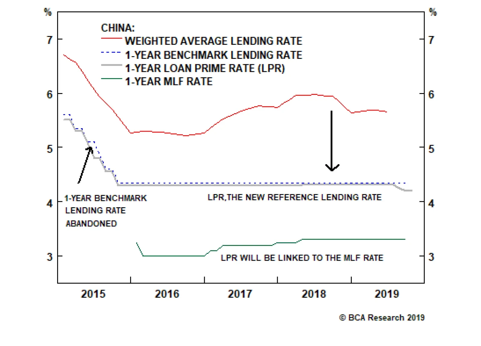Chart 5Capacity Is Not Excessively Underutilized Capacity Is Not Excessively Underutilized Capacity Is Not Excessively Underutilized Chart 6Inventory Destocking May Be Bottoming Out Inventory Destocking May Be Bottoming Out Inventory Destocking May Be Bottoming Out But the bad news (for investors), is that contained, or mild producer price deflation will not be reason alone to spur aggressive further easing from policymakers. This means that the re-emergence of price deflation, even mild and short-lived, will weigh on earnings and investor sentiment. Bottom Line: This episode of producer price deflation is unlikely to become as pernicious as occurred in the past, but policymakers are thus unlikely to act aggressively to counter it. While this removes some of the downside risks for Chinese stocks, even mild deflation will weigh on earnings growth (and thus sentiment) which underscores our tactically bearish stance on Chinese stocks. Demystifying China’s New Loan Prime Rate: Not The Stimulus You Are Looking For On August 20th, the PBoC launched a new loan prime rate (LPR) system, a revamped reference regime for setting bank loan interest rates3 (Chart 7). In September, the new LPR rate for one-year bank loans was lowered by five basis points. Since then, the market has been fixated on predicting whether the PBoC will cut the Medium-Lending Facility (MLF) rate next, which would be perceived as a change in China’s monetary stance. Chart 7China's New LPR: A Shadow 'Tax Cut' China's New LPR: A Shadow "Tax Cut" China's New LPR: A Shadow "Tax Cut" PBoC will increase its control of the pricing of credit, while tight financial regulations will restrict the size and speed of credit growth. The new LPR reform, in our view, is designed to force state-owned (and better-capitalized) commercial banks to hand out a “tax cut” to struggling small- and medium-sized enterprises (SMEs) by lowering bank lending rates. At the same time, it allows the PBoC to take back control of the pricing of credit from commercial banks, “killing two birds with one stone.” There are three main market implications from this approach: The new LPR is likely to gradually narrow the gap between corporate bond yields (i.e. “market rates”) and bank lending rates; A cut in the MLF rate in the near term should be interpreted as a “reward” to commercial banks rather than a stimulus for the economy; Most importantly, the new LPR system does not mean rapid credit expansion is in the cards. Quite the opposite, in the near term, banks may tighten their lending. The wide spread between the 3-month interbank repo rate and average bank lending rate illustrates the reason why the PBoC has introduced the LPR.4 This gap is also evident when comparing the yield of AAA-rated corporate bonds and the average bank lending rate (Chart 8). These gaps exist because Chinese commercial banks have largely manipulated the 1-year bank lending rate set by the PBoC when lending to their “preferred customers,” usually state-owned enterprises and real estate developers, by offering significantly discounted loan rates. Banks then charge substantial “risk premiums” on loans to the private sector, mostly SMEs, to make up for the narrower profit margins on loans to SOEs (Chart 9). Chart 8An Impaired Monetary Policy Transmission Mechanism An Impaired Monetary Policy Transmission Mechanism An Impaired Monetary Policy Transmission Mechanism Chart 9Evidence Of Asymmetrical Lending Practices Evidence Of Asymmetrical Lending Practices Evidence Of Asymmetrical Lending Practices The new LPR system is designed to minimize this discrepancy, since the new LPRs are more market based and are quoted based on the price of loans banks charge their prime clients. By design, the new LPR system should force the average bank lending rate closer to the rate companies borrow in the bond market. This means bank lending rates will be guided lower, including lending rates for SMEs. However, the new system will be implemented in phases, and the PBoC is likely to gradually guide LPRs lower to allow banks to readjust their pricing models.  The LPR rate is essentially the MLF rate plus bank profit margins (the added basis points above the MLF rate). The market will guide the top line lending rate, while the PBoC will have control over the floor rate (MLF) through open market operations. The fact that the PBoC is keeping the MLF rate unchanged while allowing the LPR to drop (albeit slightly) sends an explicit message: The PBoC is forcing banks to lower lending rates first before boosting their now-narrowed profit margins by lowering the MLF rate. In contrast to expectations of market participants that the LPR system will ease credit conditions, banks may actually tighten their lending in the coming months. While the PBoC will increase its control of the pricing of bank loans by the rate reform plan, the strengthening in financial regulations that has occurred over the past year will restrict the size and speed of credit growth. This combination has created more room for monetary easing without unleashing “animal spirits.” Borrowing costs to risky institutions have been higher since the Baoshang Bank takeover and are likely to remain elevated even if interest rates are lower (Chart 10). More importantly, mortgage and real estate developer loans together account for nearly 30% of total bank credit. Unless policymakers ease the brakes on lending restrictions to the property sector, bank lending growth is unlikely to pick up meaningfully (Chart 11). In fact, the PBoC has explicitly excluded mortgage and property-related lending from benefitting from the LPR rate cut.5 Barring a significant worsening in economic data, we do not expect the PBoC to lower mortgage lending and real estate-related loan rates in the coming months. Chart 10Tightened Financial Regulations Will Keep Cost Of Risky Lending High Tightened Financial Regulations Will Keep Cost Of Risky Lending High Tightened Financial Regulations Will Keep Cost Of Risky Lending High Chart 11Mortgage Rate Unlikely To Return To Its 2016 Low Mortgage Rate Unlikely To Return To Its 2016 Low Mortgage Rate Unlikely To Return To Its 2016 Low Finally, in the next two- to three-quarter mandatory implementation period, banks will be readjusting their pricing and credit risk-assessing models. During the transition, we expect more cautious sentiment among both lenders and borrowers. Hence, in the short term, bank loan growth may actually moderate. Bottom Line: The new LPR system may lower China’s banking sector profits in the short term. But in the next 6- to 12-months, we expect the PBoC to compensate commercial banks by keeping ample liquidity in the interbank system and by eventually lowering the MLF rate. The new LPR system may slow bank credit growth in the next few months, but after its full implementation (by the second quarter of 2020), it will have the potential to make PBoC’s policy more effective. Investment Conclusions We expect two phases of Chinese equity relative performance over the coming year: one phase of flat-to-potentially seriously down performance to last from now until sometime in the first quarter of 2020 when the economy bottoms, and then a phase of outperformance. Our expectation that the economy will bottom in Q1 2020 rests on the existing reflationary response by Chinese policymakers and an improved monetary transmission mechanism. Chart 12We Expect The Chinese Economy To Bottom In Q1 2020 We Expect The Chinese Economy To Bottom In Q1 2020 We Expect The Chinese Economy To Bottom In Q1 2020 Our expectation that the economy will bottom in the first quarter of 2020 continues to rest on the existing reflationary response by Chinese policymakers (Chart 12), and the fact that China’s new LPR system has the potential to improve what is currently a seriously impaired monetary transmission mechanism beyond the next two or three quarters. But the existing response of policymakers has been considerably more measured when compared to past economic cycles, meaning that equity investors are unlikely to be as forward-looking as they otherwise might be. Weak producer price deflation will weigh on investor sentiment, and it is unlikely to be weak enough to spur aggressive further easing. The potential for further escalation of the U.S.-China trade war also compellingly argues against an overweight stance in the near-term, even if we expect economic growth to subsequently improve. Consequently, we remain tactically bearish and cyclically bullish towards Chinese stocks: medium-term investors who are already positioned in favor of China-related assets should stay long, whereas investors who have not yet moved to an overweight stance should wait for a better buying opportunity to emerge over the coming few months.   Jing Sima China Strategist JingS@bcaresearch.com     Footnotes 1      Please see Global Investment Strategy Outlook “Fourth Quarter 2019 Strategy Outlook: A “Show Me” Market”, dated October 4, 2019, available at gis.bcaresearch.com 2      Please see China Investment Strategy Weekly Report “China Macro And Market Review”, dated October 2, 2019, available at cis.bcaresearch.com 3      Announcement of the People’s Bank of China on Improving Loan Prime Rate (LPR) Formation Mechanism, August 19, 2019, available at http://www.pbc.gov.cn/en/3688110/3688172/3877490/index.html 4      PBC Official Answers Press Questions on Improving Loan Prime Rate (LPR) Formation Mechanism, August 20, 2019, available at http://www.pbc.gov.cn/en/3688110/3688172/3877865/index.html 5      Announcement of the People’s Bank of China No.16, August 27, 2019, available at http://www.pbc.gov.cn/en/3688110/3688172/3881177/index.html Cyclical Investment Stance Equity Sector Recommendations

Highlights The Cold War is a limited analogy for the U.S.-China conflict; In a multipolar world, complete bifurcation of trade is difficult if not impossible; History suggests that trade between rivals will continue, with minimal impediments; On a secular horizon, buy defense stocks, Europe, capex, and non-aligned countries. Feature There is a growing consensus that China and the U.S. are hurtling towards a Cold War. BCA Research played some part in this consensus – at least as far as the investment community is concerned – by publishing “Power and Politics in East Asia: Cold War 2.0?” in September 2012.1 For much of this decade, Geopolitical Strategy focused on the thesis that geopolitical risk was rotating out of the Middle East, where it was increasingly irrelevant, to East Asia, where it would become increasingly relevant. This thesis remains cogent, but it does not mean that a “Silicon Curtain” will necessarily divide the world into two bifurcated zones of capitalism. Trade, capital flows, and human exchanges between China and the U.S. will continue and may even grow. But the risk of conflict, including a military one, will not decline. In this report, we first review the geopolitical logic that underpins Sino-American tensions. We then survey the academic literature for clues on how that relationship will develop vis-à-vis trade and economic relations. The evidence from political theory is surprising and highly investment relevant. We then look back at history for clues as to what this means for investors. Our conclusion is that it is highly likely that the U.S. and China will continue to be geopolitical rivals. However, due to the geopolitical context of multipolarity, it is unlikely that the result will be “Bifurcated Capitalism.” Rather, we expect an exciting and volatile environment for investors where geopolitics takes its historical place alongside valuation, momentum, fundamentals, and macroeconomics in the pantheon of factors that determine investment opportunities and risks. The Thucydides Trap Is Real … Speaking in the Reichstag in 1897, German Foreign Secretary Bernhard von Bülow proclaimed that it was time for Germany to demand “its own place in the sun.”2 The occasion was a debate on Germany’s policy towards East Asia. Bülow soon ascended to the Chancellorship under Kaiser Wilhelm II and oversaw the evolution of German foreign policy from Realpolitik to Weltpolitik. While Realpolitik was characterized by Germany’s cautious balancing of global powers under Chancellor Otto von Bismarck, Weltpolitik saw Bülow and Wilhelm II seek to redraw the status quo through aggressive foreign and trade policy. Imperial Germany joined a long list of antagonists, from Athens to today’s People’s Republic of China, in the tragic play of human history dubbed the “Thucydides Trap.”3 Chart 1Imperial Overstretch Imperial Overstretch Imperial Overstretch The underlying concept is well known to all students of world history. It takes its name from the Greek historian Thucydides and his seminal History of the Peloponnesian War. Thucydides explains why Sparta and Athens went to war but, unlike his contemporaries, he does not moralize or blame the gods. Instead, he dispassionately describes how the conflict between a revisionist Athens and established Sparta became inevitable due to a cycle of mistrust. Graham Allison, one of America’s preeminent scholars of international relations, has argued that the interplay between a status quo power and a challenger has almost always led to conflict. In 12 out of the 16 cases he surveyed, actual military conflict broke out. Of the four cases where war did not develop, three involved transitions between countries that shared a deep cultural affinity and a respect for the prevailing institutions.4 In those cases, the transition was a case of new management running largely the same organizational structure. And one of the four non-war outcomes was nothing less than the Cold War between the Soviet Union and the U.S. The fundamental problem for a status quo power is that its empire or “sphere of influence” remains the same size as when it stood at the zenith of power. However, its decline in a relative sense leads to a classic problem of “imperial overstretch.” The hegemonic or imperial power erroneously doubles down on maintaining a status quo that it can no longer afford (Chart 1). The challenger power is not blameless. It senses weakness in the hegemon and begins to develop a regional sphere of influence. The problem is that regional hegemony is a perfect jumping off point towards global hegemony. And while the challenger’s intentions may be limited and restrained (though they often are ambitious and overweening), the status quo power must react to capabilities, not intentions. The former are material and real, whereas the latter are perceived and ephemeral. The challenging power always has an internal logic justifying its ambitions. In China’s case today, there is a sense among the elite that the country is merely mean-reverting to the way things were for many centuries in China’s and Asia’s long history (Chart 2). In other words, China is a “challenger” power only if one describes the status quo as the past three hundred years. It is the “established” power if one goes back to an earlier state of affairs. As such, the consensus in China is that it should not have to pay deference to the prevailing status quo given that the contemporary context is merely the result of western imperialist “challenges” to the established Chinese and regional order. 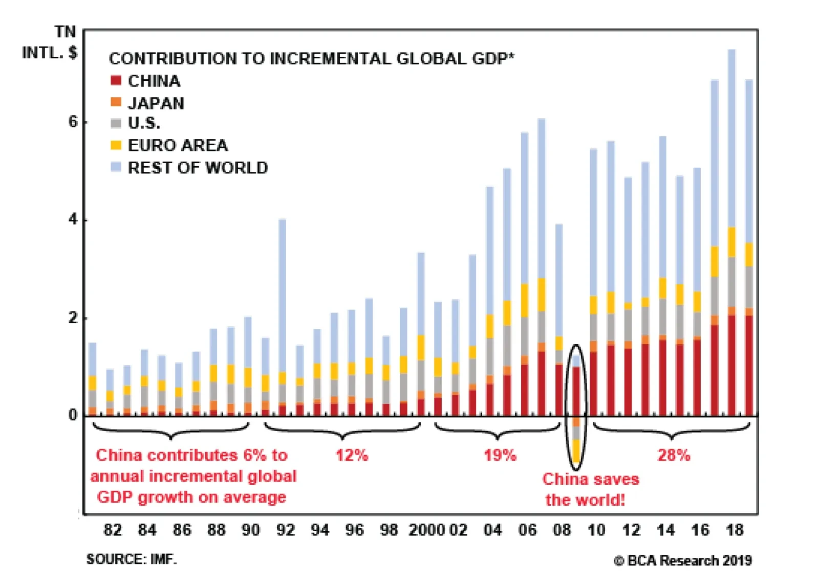Chart 2China’s Mean Reverting Narrative Back To The Nineteenth Century Back To The Nineteenth Century In addition, China has a legitimate claim that it is at least as relevant to the global economy as the U.S. and therefore deserves a greater say in global governance. While the U.S. still takes a larger share of the global economy, China has contributed 23% to incremental global GDP over the past two decades, compared to 13% for the U.S. (Chart 3). Chart 3The Beijing Consensus Back To The Nineteenth Century Back To The Nineteenth Century Bottom Line: The emerging tensions between China and the U.S. fit neatly into the theoretical and empirical outlines of the Thucydides Trap. We do not see any way for the two countries to avoid struggle and conflict on a secular or forecastable horizon. What does this mean for investors? For one, the secular tailwinds behind defense stocks will persist. But what beyond that? Is the global economy destined to witness complete bifurcation into two armed camps separated by a Silicon Curtain? Will the Alibaba and Amazon Pacts suspiciously glare at each other the way that NATO and Warsaw Pacts did amidst the Cold War? The answer, tentatively, is no. … But It Will Not Lead to Economic Bifurcation President Trump’s aggressive trade policy also fits neatly into political theory, to a point. Realism in political science focuses on relative gains over absolute gains in all relationships, including trade. This is because trade leads to economic prosperity, prosperity to the accumulation of economic surplus, and economic surplus to military spending, research, and development. Two states that care only about relative gains due to rivalry produce a zero-sum game with no room for cooperation. It is a “Prisoner’s Dilemma” that can lead to sub-optimal economic outcomes in which both actors chose not to cooperate. The U.S.-China conflict will not lead to complete bifurcation of the global economy. Diagram 1 illustrates the effects of relative gain calculations on the trade behavior of states. In the absence of geopolitics, demand (Q3) is satisfied via trade (Q3-Q0) due to the inability of domestic production (Q0) to meet it. Diagram 1Trade War In A Bipolar World Back To The Nineteenth Century Back To The Nineteenth Century However, geopolitical externality – a rivalry with another state – raises the marginal social cost of imports – i.e. trade allows the rival to gain more out of trade and “catch up” in terms of geopolitical capabilities. The trading state therefore eliminates such externalities with a tariff (t), raising domestic output to Q1, while shrinking demand to Q2, thus reducing imports to merely Q2-Q1, a fraction of where they would be in a world where geopolitics do not matter. The dynamic of relative gains can also have a powerful pull on the hegemon as it begins to weaken and rethink its originally magnanimous trade relations. As political scientist Duncan Snidal argued in a 1991 paper, When the global system is first set up, the hegemon makes deals with smaller states. The hegemon is concerned more with absolute gains, smaller states are more concerned with relative, so they are tougher negotiators. Cooperative arrangements favoring smaller states contribute to relative hegemonic decline. As the unequal distribution of benefits in favor of smaller states helps them catch up to the hegemonic actor, it also lowers the relative gains weight they place on the hegemonic actor. At the same time, declining relative preponderance increases the hegemonic state’s concern for relative gains with other states, especially any rising challengers. The net result is increasing pressure from the largest actor to change the prevailing system to gain a greater share of cooperative benefits.5 The reason small states are initially more concerned with relative gains is because they are far more concerned with national security than the hegemon. The hegemon has a preponderance of power and is therefore more relaxed about its security needs. This explains why Presidents George Bush Sr., Bill Clinton, and George Bush Jr. all made “bad deals” with China. Writing nearly thirty years ago, Snidal cogently described the current U.S.-China trade war. Snidal thought he was describing a coming decade of anarchy. But he and fellow political scientists writing in the early 1990s underestimated American power. The “unipolar moment” of American supremacy was not over, it was just beginning! As such, the dynamic Snidal described took thirty years to come to fruition. When thinking about the transition away from U.S. hegemony, most investors anchor themselves to the Cold War as it is the only world they have known that was not unipolar. Moreover the Cold War provides a simple, bipolar distribution of power that is easy to model through game theory. If this is the world we are about to inhabit, with the U.S. and China dividing the whole planet into spheres like the U.S. and Soviet Union, then the paragraph we lifted from Snidal’s paper would be the end of it. America would abandon globalization in totality, impose a draconian Silicon Curtain around China, and coerce its allies to follow suit. But most of recent human history has been defined by a multipolar distribution of power between states, not a bipolar one. The term “cold war” is applicable to the U.S. and China in the sense that comparable military power may prevent them from fighting a full-blown “hot war.” But ultimately the U.S.-Soviet Cold War is a poor analogy for today’s world. In a multipolar world, Snidal concludes, “states that do not cooperate fall behind other relative gains maximizers that cooperate among themselves. This makes cooperation the best defense (as well as the best offense) when your rivals are cooperating in a multilateral relative gains world.” Snidal shows via formal modeling that as the number of players increases from two, relative-gains sensitivity drops sharply.6 The U.S.-China relationship does not occur in a vacuum — it is moderated by the global context. Today’s global context is one of multipolarity. Multipolarity refers to the distribution of geopolitical power, which is no longer dominated by one or two great powers (Chart 4). Europe and Japan, for instance, have formidable economies and military capabilities. Russia remains a potent military power, even as India surpasses it in terms of overall geopolitical power. Chart 4The World Is No Longer Bipolar The World Is No Longer Bipolar The World Is No Longer Bipolar A multipolar world is the least “ordered” and the most unstable of world systems (Chart 5). This is for three reasons: Chart 5Multipolarity Is Messy Multipolarity Is Messy Multipolarity Is Messy Math: Multipolarity engenders more potential “conflict dyads” that can lead to conflict. In a unipolar world, there is only one country that determines norms and rules of behavior. Conflict is possible, but only if the hegemon wishes it. In a bipolar world, conflict is possible, but it must align along the axis of the two dominant powers. In a multipolar world, alliances are constantly shifting and producing novel conflict dyads. Lack of coordination: Global coordination suffers in periods of multipolarity as there are more “veto players.” This is particularly problematic during times of stress, such as when an aggressive revisionist power uses force or when the world is faced with an economic crisis. Charles Kindleberger has argued that it was exactly such hegemonic instability that caused the Great Depression to descend into the Second World War in his seminal The World In Depression.7 Mistakes: In a unipolar and bipolar world, there are a very limited number of dice being rolled at once. As such, the odds of tragic mistakes are low and can be mitigated with complex formal relationships (such as U.S.-Soviet Mutually Assured Destruction, grounded in formal modeling of game theory). But in a multipolar world, something as random as an assassination of a dignitary can set in motion a global war. The multipolar system is far more dynamic and thus unpredictable. In a multipolar world, the U.S. will not be able to exclude China from the global system. Diagram 2 is modified for a multipolar world. Everything is the same, except that we highlight the trade lost to other great powers. The state considering using tariffs to lower the marginal social cost of trading with a rival must account for this “lost trade.” In the context of today’s trade war with China, this would be the sum of all European Airbuses and Brazilian soybeans sold to China in the place of American exports. For China, it would be the sum of all the machinery, electronics, and capital goods produced in the rest of Asia and shipped to the United States. Diagram 2Trade War In A Multipolar World Back To The Nineteenth Century Back To The Nineteenth Century Could Washington ask its allies – Europe, Japan, South Korea, Taiwan, etc. – not to take advantage of the lucrative trade (Q3-Q0)-(Q2-Q1) lost due to its trade tiff with China? Sure, but empirical research shows that they would likely ignore such pleas for unity. Alliances produced by a bipolar system produce a statistically significant and large impact on bilateral trade flows, a relationship that weakens in a multipolar context. This is the conclusion of a 1993 paper by Joanne Gowa and Edward D. Mansfield.8 The authors draw their conclusion from an 80-year period beginning in 1905, which captures several decades of global multipolarity. Unless the U.S. produces a wholehearted diplomatic effort to tighten up its alliances and enforce trade sanctions – something hardly foreseeable under the current administration – the self-interest of U.S. allies will drive them to continue trading with China. The U.S. will not be able to exclude China from the global system; nor will China be able to achieve Xi Jinping’s vaunted “self-sufficiency.” A risk to our view is that we have misjudged the global system, just as political scientists writing in the early 1990s did. To that effect, we accept that Charts 1 and 4 do not really support a view that the world is in a balanced multipolar state. The U.S. clearly remains the most powerful country in the world. The problem is that it is also clearly in a relative decline and that its sphere of influence is global – and thus very expensive – whereas its rivals have merely regional ambitions (for the time being). As such, we concede that American hegemony could be reasserted relatively quickly, but it would require a significant calamity in one of the other poles of power. For instance, a breakdown in China’s internal stability alongside the recovery of U.S. political stability. Bottom Line: The trade war between the U.S. and China is geopolitically unsustainable. The only way it could continue is if the two states existed in a bipolar world where the rest of the states closely aligned themselves behind the two superpowers. We have a high conviction view that today’s world is – for the time being – multipolar. American allies will cheat and skirt around Washington’s demands that China be isolated. This is because the U.S. no longer has the preponderance of power that it enjoyed in the last decade of the twentieth and the first decade of the twenty-first century. Insights presented thus far come from formal theory in political science. What does history teach us? Trading With The Enemy In 1896, a bestselling pamphlet in the U.K., “Made in Germany,” painted an ominous picture: “A gigantic commercial State is arising to menace our prosperity, and contend with us for the trade of the world.”9 Look around your own houses, author E.E. Williams urged his readers. “The toys, and the dolls, and the fairy books which your children maltreat in the nursery are made in Germany: nay, the material of your favorite (patriotic) newspaper had the same birthplace as like as not.” Williams later wrote that tariffs were the answer and that they “would bring Germany to her knees, pleading for our clemency.”10 By the late 1890s, it was clear to the U.K. that Germany was its greatest national security threat. The Germany Navy Laws of 1898 and 1900 launched a massive naval buildup with the singular objective of liberating the German Empire from the geographic constraints of the Jutland Peninsula. By 1902, the First Lord of the Royal Navy pointed out that “the great new German navy is being carefully built up from the point of view of a war with us.”11 There is absolutely no doubt that Germany was the U.K.’s gravest national security threat. As a result, London signed in April 1904 a set of agreements with France that came to be known as Entente Cordiale. The entente was immediately tested by Germany in the 1905 First Moroccan Crisis, which only served to strengthen the alliance. Russia was brought into the pact in 1907, creating the Triple Entente. In hindsight, the alliance structure was obvious given Germany’s meteoric rise from unification in 1871. However, one should not underestimate the magnitude of these geopolitical events. For the U.K. and France to resolve centuries of differences and formalize an alliance in 1904 was a tectonic shift — one that they undertook against the grain of history, entrenched enmity, and ideology.12 History teaches us that trade occurs even amongst rivals and during wartime. Political scientists and historians have noted that geopolitical enmity rarely produces bifurcated economic relations exhibited during the Cold War. Both empirical research and formal modeling shows that trade occurs even amongst rivals and during wartime.13 This was certainly the case between the U.K. and Germany, whose trade steadily increased right up until the outbreak of World War One (Chart 6). Could this be written off due to the U.K.’s ideological commitment to laissez-faire economics? Or perhaps London feared a move against its lightly defended colonies in case it became protectionist? These are fair arguments. However, they do not explain why Russia and France both saw ever-rising total trade with the German Empire during the same period (Chart 7). Either all three states were led by incompetent policymakers who somehow did not see the war coming – unlikely given the empirical record – or they simply could not afford to lose out on the gains of trade with Germany to each other. Chart 6The Allies Traded With Germany… Back To The Nineteenth Century Back To The Nineteenth Century Chart 7… Right Up To WWI Back To The Nineteenth Century Back To The Nineteenth Century Chart 8Japan And U.S. Never Downshifted Trade Back To The Nineteenth Century Back To The Nineteenth Century A similar dynamic was afoot ahead of World War Two. Relations between the U.S. and Japan soured in the 1930s, with the Japanese invasion of Manchuria in 1931. In 1935, Japan withdrew from the 1922 Washington Naval Treaty – the bedrock of the Pacific balance of power – and began a massive naval buildup. In 1937, Japan invaded China. Despite a clear and present danger, the U.S. continued to trade with Japan right up until July 26, 1941, few days after Japan invaded southern Indochina (Chart 8). On December 7, Japan attacked the U.S. A skeptic may argue that precisely because policymakers sleepwalked into war in the First and Second World Wars, they will not (or should not) make the same mistake this time around. First, we do not make policy prescriptions and therefore care not what should happen. Second, we are highly skeptical of the view that policymakers in the early and mid-twentieth century were somehow defective (as opposed to today’s enlightened leaders). Our constraints-based framework urges us to seek systemic reasons for the behavior of leaders. Political science provides a clear theoretical explanation for why London and Washington continued to trade with the enemy despite the clarity of the threat. The answer lies in the systemic nature of the constraint: a multipolar world reduces the sensitivity of policymakers to relative gains by introducing a collective action problem thanks to changing alliances and the difficulty of disciplining allies’ behavior. In the case of U.S. and China, this is further accentuated by President Trump’s strategy of skirting multilateral diplomacy and intense focus on mercantilist measures of power (i.e. obsession with the trade deficit). An anti-China trade policy that was accompanied by a magnanimous approach to trade relations with allies could have produced a “coalition of the willing” against Beijing. But after two years of tariffs and threats against the EU, Japan, and Canada, the Trump administration has already signaled to the rest of the world that old alliances and coordination avenues are up for revision. There are two outcomes that we can see emerging over the course of the next decade. First, U.S. leadership will become aware of the systemic constraints under which they operate, and trade with China will continue – albeit with limitations and variations. However, such trade will not reduce the geopolitical tensions, nor will it prevent a military conflict. In facts, the probability of military conflict may increase even as trade between China and the U.S. remains steady. Second, U.S. leadership will fail to correctly assess that they operate in a multipolar world and will give up the highlighted trade gains from Diagram 2 to economic rivals such as Europe and Japan. Given our methodological adherence to constraint-based forecasting, we highly doubt that the latter scenario is likely. Bottom Line: The China-U.S. conflict is not a replay of the Cold War. Systemic pressures from global multipolarity will force the U.S. to continue to trade with China, with limitations on exchanges in emergent, dual-use technologies that China will nonetheless source from other technologically advanced countries. This will create a complicated but exciting world where geopolitics will cease to be seen as exogenous to investing. A risk to the sanguine conclusion is that the historical record is applicable to today, but that the hour is late, not early. It is already July 26, 1941 – when U.S. abrogated all trade with Japan – not 1930. As such, we do not have another decade of trade between U.S. and China remaining, we are at the end of the cycle. While this is a risk, it is unlikely. American policymakers would essentially have to be willing to risk a military conflict with China in order to take the trade war to the same level they did with Japan. It is an objective fact that China has meaningfully stepped up aggressive foreign policy in the region. But unlike Japan in 1941, China has not outright invaded any countries over the past decade. As such, the willingness of the public to support such a conflict is unclear, with only 21% of Americans considering China a top threat to the U.S. Investment Implications This analysis is not meant to be optimistic. First, the U.S. and China will continue to be rivals even if the economic relationship between them does not lead to global bifurcation. For one, China continues to be – much like Germany in the early twentieth century – concerned with access to external markets on which 19.5% of its economy still depend. China is therefore developing a modern navy and military not because it wants to dominate the rest of the world but because it wants to dominate its near abroad, much as the U.S. wanted to, beginning with the Monroe Doctrine. This will continue to lead to Chinese aggression in the South and East China Seas, raising the odds of a conflict with the U.S. Navy. Given that the Thucydides Trap narrative remains cogent, investors should look to overweight S&P 500 aerospace and defense stocks relative to global equity markets. An alternative way that one could play this thesis is by developing a basket of global defense stocks. Multipolarity may create constraints to trade protectionism, but it engenders geopolitical volatility and thus buoys defense spending. Second, we would not expect another uptick in globalization. Multipolarity may make it difficult for countries to completely close off trade with a rival, but globalization is built on more than just trade between rivals. Globalization requires a high level of coordination among great powers that is only possible under hegemonic conditions. Chart 9 shows that the hegemony of the British and later American empires created a powerful tailwind for trade over the past two hundred years. Chart 9The Apex Of Globalization Is Behind Us The Apex Of Globalization Is Behind Us The Apex Of Globalization Is Behind Us The Apex of Globalization has come and gone – it is all downhill from here. But this is not a binary view. Foreign trade will not go to zero. The U.S. and China will not completely seal each other’s sphere of influence behind a Silicon Curtain. Instead, we focus on five investment themes that flow from a world that is characterized by the three trends of multipolarity, Sino-U.S. geopolitical rivalry, and apex of globalization: Europe will profit: As the U.S. and China deepen their enmity, we expect some European companies to profit. There is some evidence that the investment community has already caught wind of this trend, with European equities modestly outperforming their U.S. counterparts whenever trade tensions flared up in 2019 (Chart 10). Given our thesis, however, it is unlikely that the U.S. would completely lose market share in China to Europe. As such, we specifically focus on tech, where we expect the U.S. and China to ramp up non-tariff barriers to trade regardless of systemic pressures to continue to trade. A strategic long in the secularly beleaguered European tech companies relative to their U.S. counterparts may therefore make sense (Chart 11). Chart 10Europe: A Trade War Safe Haven Europe: A Trade War Safe Haven Europe: A Trade War Safe Haven Chart 11Is Europe Really This Incompetent? Is Europe Really This Incompetent? Is Europe Really This Incompetent? USD bull market will end: A trade war is a very disruptive way to adjust one’s trade relationship. It opens one to retaliation and thus the kind of relative losses described in this analysis. As such, we expect that U.S. to eventually depreciate the USD, either by aggressively reversing 2018 tightening or by coercing its trade rivals to strengthen their currencies. Such a move will be yet another tailwind behind the diversification away from the USD as a reserve currency, a move that should benefit the euro. Bull market in capex: The re-wiring of global manufacturing chains will still take place. The bad news is that multinational corporations will have to dip into their profit margins to move their supply chains to adjust to the new geopolitical reality. The good news is that they will have to invest in manufacturing capex to accomplish the task. One way to articulate this theme is to buy an index of semiconductor capital companies (AMAT, LRCX, KLAC, MKSI, AEIS, BRIKS, and TER). Given the highly cyclical nature of capital companies, we would recommend an entry point once trade tensions subside and green shoots of global growth appear. “Non-aligned” markets will benefit: The last time the world was multipolar, great powers competed through imperialism. This time around, a same dynamic will develop as countries seek to replicate China’s “Belt and Road Initiative.” This is positive for frontier markets. A rush to provide them with exports and services will increase supply and thus lower costs, providing otherwise forgotten markets with a boon of investments. India, and Asia-ex-China more broadly, stand as intriguing alternatives to China, especially with the current administration aggressively reforming to take advantage of the rewiring of global manufacturing chains. Capital markets will remain globalized: With interest rates near zero in much of the developed world and the demographic burden putting an ever-greater pressure on pension plans to generate returns, the search for yield will continue to be a powerful drive that keeps capital markets globalized. Limitations are likely to grow, especially when it comes to cross-border private investments in dual-use technologies. But a completely bifurcation of capital markets is unlikely. The world we are describing is one where geopolitics will play an increasingly prominent role for global investors. It would be convenient if the world simply divided into two warring camps, leaving investors with neatly separated compartments that enabled them to go back to ignoring geopolitics. This is unlikely. Rather, the world will resemble the dynamic years at the end of the nineteenth century, a rough-and-tumble era that required a multi-disciplinary approach to investing.   Marko Papic, Consulting Editor, BCA Research Chief Strategist, Clocktower Group Marko@clocktowergroup.com Footnotes 1 Please see BCA Research Geopolitical Strategy, “Power And Politics In East Asia: Cold War 2.0?,” September 25, 2012, “Sino-American Conflict: More Likely Than You Think,” October 4, 2013, “The Great Risk Rotation,” December 11, 2013, and “Strategic Outlook 2014 – Stay The Course: EM Risk – DM Reward,” January 23, 2014, “Underestimating Sino-American Tensions,” November 6, 2015, “The Geopolitics Of Trump,” December 2, 2016, “How To Play The Proxy Battles In Asia,” March 1, 2017, and others available at gps.bcaresearch.com or upon request. 2 Please see German Historical Institute, “Bernhard von Bulow on Germany’s ‘Place in the Sun’” (1897), available at http://germanhistorydocs.ghi-dc.org/ 3 See Graham Allison, Destined For War: Can America and China Escape Thucydides’s Trap? (New York: Houghton Miffin Harcourt, 2017). 4 The three cases are Spain taking over from Portugal in the sixteenth century, the U.S. taking over from the U.K. in the twentieth century, and Germany rising to regional hegemony in Europe in the twenty-first century. 5 Duncan Snidal, “Relative Gains and the Pattern of International Cooperation,” The American Political Science Review, 85:3 (September 1991), pp. 701-726. 6 We do not review Snidal’s excellent game theory formal modeling in this paper as it is complex and detailed. However, we highly encourage the intrigued reader to pursue the study on their own. 7 See Charles P. Kindleberger, The World In Depression, 1929-1939 (Berkeley: University of California Press, 2013). 8 Joanne Gowa and Edward D. Mansfield, “Power Politics and International Trade,” The American Political Science Review, 87:2 (June 1993), pp. 408-420. 9 See Ernest Edwin Williams, Made in Germany (reprint, Ithaca: Cornell University Press), available at https://archive.org/details/cu31924031247830. 10 Quoted in Margaret MacMillan, The War That Ended Peace (Toronto: Allen Lane, 2014). 11 Peter Liberman, “Trading with the Enemy: Security and Relative Economic Gains,” international Security, 21:1 (Summer 1996), pp. 147-175. 12 Although France and Russia overcame even greater bitterness due to the ideological differences between a republic founded on a violent uprising against its aristocracy – France – and an aristocratic authoritarian regime – Russia. 13 See James Morrow, “When Do ‘Relative Gains’ Impede Trade?” The Journal of Conflict Resolution, 41:1 (February 1997), pp. 12-37; and Jack S. Levy and Katherine Barbieri, “Trading With the Enemy During Wartime,” Security Studies, 13:3 (December 2004), pp. 1-47.

Highlights MARKET FORECASTS Fourth Quarter 2019 Strategy Outlook: A "Show Me" Market Fourth Quarter 2019 Strategy Outlook: A "Show Me" Market Investment Strategy: Markets have entered a “show me” phase. Better economic data and meaningful progress on the trade negotiations will be necessary for stocks to move sustainably higher. We think both preconditions will be realized. Until then, risk assets could come under pressure. Global Asset Allocation: Investors should overweight stocks relative to bonds over a 12-month horizon, but maintain higher-than-normal cash positions in the near term as a hedge against downside risks. Equities: EM and European stocks will outperform once global growth bottoms out. Cyclical sectors, including financials, will also start to outperform defensives when the growth cycle turns. Bonds: Central banks will remain dovish, but yields will nevertheless rise modestly on the back of stronger global growth. Favor high-yield corporate credit over government bonds. Currencies: As a countercyclical currency, the U.S. dollar should peak later this year. Commodities: Oil and industrial metals prices will move higher. Gold prices have entered a holding pattern, but should shine again late next year or in 2021 when inflation finally breaks out. Feature Dear Client, In lieu of this report, I hosted a webcast on Monday, October 7th at 10:00 AM EDT, where I discussed the major investment themes and views I see playing out for the rest of the year and beyond. Best regards, Peter Berezin, Chief Global Strategist   I. Global Macro Outlook A Testing Phase For The Global Economy The global economy has reached a critical juncture. Growth has been slowing since early 2018, reaching what many would regard as “stall speed.” This is the point where economic weakness begins to feed on itself, potentially triggering a recession. Will the growth slowdown worsen? Our guess is that it won’t. Global financial conditions have eased significantly over the past four months, thanks in part to the dovish pivot by most central banks. Looser financial conditions usually bode well for global growth (Chart 1). Our global leading indicator has hooked up, mainly due to a marginal improvement in emerging markets’ data (Chart 2). Chart 1Easier Financial Conditions Will Boost Global Growth Easier Financial Conditions Will Boost Global Growth Easier Financial Conditions Will Boost Global Growth Chart 2Global LEI Has Moved Off Its Lows Global LEI Has Moved Off Its Lows Global LEI Has Moved Off Its Lows     An important question is whether the weakness in the manufacturing sector will spread to the much larger services sector. There is some evidence that this is happening, with yesterday’s weaker-than-expected ISM non-manufacturing release being the latest example. Nevertheless, the deceleration in service sector activity has been limited so far (Chart 3). Even in Germany, with its large manufacturing base, the service sector PMI remains in expansionary territory. This is a key difference with the 2001/02 and 2008/09 periods, when service sector activity collapsed in lockstep with manufacturing activity. Chart 3AThe Service Sector Has Softened Less Than Manufacturing (I) The Service Sector Has Softened Less Than Manufacturing (I) The Service Sector Has Softened Less Than Manufacturing (I) Chart 3BThe Service Sector Has Softened Less Than Manufacturing (II) The Service Sector Has Softened Less Than Manufacturing (II) The Service Sector Has Softened Less Than Manufacturing (II) The Drive-By Slowdown If one were to ask most investors the reasons behind the manufacturing slowdown, they would probably cite the trade war or the Chinese deleveraging campaign. These are both valid reasons, but there is a less well-known culprit: autos. According to WardsAuto, global auto sales fell by over 5% in the first half of the year, by far the biggest decline since the Great Recession (Chart 4). Production dropped by even more. Chart 4Weakness In The Auto Sector Has Exacerbated The Manufacturing Downturn Weakness In The Auto Sector Has Exacerbated The Manufacturing Downturn Weakness In The Auto Sector Has Exacerbated The Manufacturing Downturn Chart 5U.S. Auto Demand Is Recovering U.S. Auto Demand Is Recovering U.S. Auto Demand Is Recovering   The weakness in the global auto sector reflects a variety of factors. New stringent emission requirements, expiring tax breaks, lagged effects from tighter auto loan lending standards, and trade tensions have all played a role. In addition, the decline in gasoline prices in 2015/16 probably brought forward some automobile purchases. This suggests that the 2015/16 global manufacturing downturn may have helped sow the seeds for the current one. The fact that automobile output is falling faster than sales is encouraging because it means that excess inventories are being worked off. U.S. auto loan lending standards have started to normalize, with banks reporting stronger demand for auto loans in the latest Senior Loan Officer Survey (Chart 5). In China, auto sales have troughed after having declined by as much as 14% earlier this year (Chart 6). The Chinese automobile ownership rate is a fifth of what it is in the U.S., a quarter of what it is in Japan, and a third of what it is in Korea (Chart 7). Given the low starting point, Chinese auto sales are likely to resume their secular uptrend. Chart 6Auto Sector In China Is Finding A Floor Auto Sector In China Is Finding A Floor Auto Sector In China Is Finding A Floor Chart 7China: Structural Outlook For Autos Is Bright China: Structural Outlook For Autos Is Bright China: Structural Outlook For Autos Is Bright   The Trade War: Tracking Towards A Détente? Chart 8A Fairly Regular Three-Year Manufacturing Cycle A Fairly Regular Three-Year Manufacturing Cycle A Fairly Regular Three-Year Manufacturing Cycle Manufacturing cycles typically last about three years – 18 months of slowing growth followed by 18 months of rising growth (Chart 8). To the extent that the global manufacturing PMI peaked in the first half of 2018, we should be nearing the end of the current downturn. Of course, much depends on policy developments. As we go to press, high-level negotiations between the U.S. and China have resumed. While it is impossible to predict the outcome of these talks, it does appear that both sides have an incentive to de-escalate the trade conflict. President Trump gets much better marks from voters on his management of the economy than on anything else, including his handling of trade negotiations with China (Chart 9). A protracted trade war would hurt U.S. growth, while weakening the stock market. Both would undermine Trump’s re-election prospects. Chart 9Trump Gets Reasonably High Marks On His Handling Of The Economy, But Not Much Else Fourth Quarter 2019 Strategy Outlook: A "Show Me" Market Fourth Quarter 2019 Strategy Outlook: A "Show Me" Market Chart 10Who Will Win The 2020 Democratic Nomination? Fourth Quarter 2019 Strategy Outlook: A "Show Me" Market Fourth Quarter 2019 Strategy Outlook: A "Show Me" Market China also wants to bolster growth. As difficult as it has been for the Chinese leadership to deal with Donald Trump, trying to secure a trade deal with him after he has been re-elected would be even more challenging. This would especially be the case if Trump thought that the Chinese had tried to sabotage his re-election bid. Even if Trump were to lose the election, it is not clear that China would end up with someone more pliant to deal with on trade matters. Does the Chinese government really want to negotiate over environmental standards and human rights with President Warren, who betting markets now think has a better chance of becoming the Democratic nominee than Joe Biden (Chart 10)? The Democrats’ initiative to impeach President Trump make a trade resolution somewhat more likely. First, it brings attention to Joe Biden’s (and his son’s) own dubious dealings in Ukraine, thus delivering a blow to China’s preferred U.S. presidential candidate. Second, it makes Trump more inclined to want to put the China spat behind him in order to focus his energies on domestic matters. More Chinese Stimulus? Strategically, China has a strong incentive to stimulate its economy in order to prop up growth and gain greater leverage in the trade negotiations. The Chinese credit impulse bottomed in late 2018. The impulse leads Chinese nominal manufacturing output and most other activity indicators by about nine months (Chart 11). So far, the magnitude of China’s credit/fiscal easing has come nowhere close to matching the stimulus that was unleashed on the economy both in 2015/16 and 2008/09. This is partly because the authorities are more worried about excessive debt levels today than they were back then, but it is also because the economy is in better shape. The shock from the trade war has not been nearly as bad as the Great Recession – recall that Chinese exports to the U.S. are only 2.7% of GDP in value-added terms. Unlike in 2015/16, when China lost over $1 trillion in external reserves, capital outflows have remained muted this time around (Chart 12). Chart 11Chinese Stimulus Should Boost Global Growth Chinese Stimulus Should Boost Global Growth Chinese Stimulus Should Boost Global Growth Chart 12China: No Major Capital Outflows China: No Major Capital Outflows China: No Major Capital Outflows Better-than-expected Chinese PMI data released earlier this week offers a glimmer of hope. Nevertheless, in light of the disappointing August activity numbers, China is likely to increase the pace of stimulus in the coming months. The authorities have already reduced bank reserve requirements. We expect them to cut policy rates further in the coming months. They will also front-load local government bond issuance, which should help boost infrastructure spending. European Growth Should Improve A pickup in global growth will help Europe later this year. Germany, with its trade-dependent economy, will benefit the most. Chart 13Spreads Have Come In Across Southern Europe Spreads Have Come In Across Southern Europe Spreads Have Come In Across Southern Europe Chart 14Faster Money Growth Bodes Well For GDP Growth In The Euro Area Faster Money Growth Bodes Well For GDP Growth In The Euro Area Faster Money Growth Bodes Well For GDP Growth In The Euro Area Falling sovereign spreads should also support Southern Europe (Chart 13). The Italian 10-year spread with German bunds has narrowed by almost a full percentage point since mid-August, taking the Italian 10-year yield down to 0.83%. Greek 10-year bonds are now yielding less than U.S. Treasurys (the Greek manufacturing PMI is currently the strongest in the world). With the ECB back in the market buying sovereign and corporate debt, borrowing rates should remain low. Euro area money growth, which leads GDP growth, has already picked up (Chart 14). Bank lending to the private sector should continue to accelerate. A modest serving of fiscal stimulus will also help. The European Commission estimates that the fiscal thrust in the euro area will increase by 0.5% of GDP in 2019 (Chart 15). Assuming, conservatively, a fiscal multiplier of one, this would boost euro area growth by half a percentage point. Owing to lags between changes in fiscal policy and their impact on the real economy, most of the gains to GDP growth will occur over the remainder of this year and in 2020. Chart 15Euro Area Fiscal Stimulus Will Also Boost Growth Euro Area Fiscal Stimulus Will Also Boost Growth Euro Area Fiscal Stimulus Will Also Boost Growth Chart 17Brexit Angst: A Case Of Bremorse Brexit Angst: A Case Of Bremorse Brexit Angst: A Case Of Bremorse Chart 16U.K.: Brexit Uncertainty Is Weighing On Growth U.K.: Brexit Uncertainty Is Weighing On Growth U.K.: Brexit Uncertainty Is Weighing On Growth In the U.K., Brexit uncertainty continues to weigh on growth. U.K. business investment has been especially hard hit (Chart 16). Prime Minister Boris Johnson remains insistent that he will take the U.K. out of the EU with or without a deal at the end of October. We would downplay his bluster. The Supreme Court has already denied his attempt to shutter parliament. The public is having second thoughts about the desirability of Brexit (Chart 17). While we do not have a strong view on the exact plot twists in the Brexit saga, we maintain that the odds of a no-deal Brexit are low. This is good news for U.K. growth and the pound. Japan: Own Goal Recent Japanese data releases have not been encouraging: Machine tool orders declined by 37% year-over-year in August. Exports contracted by over 8%, with imports recording a drop of 12%. The September PMI print exposed further deterioration in manufacturing, with the index falling to 48.9 from 49.3 in August. In addition, industrial production contracted by more than expected in August, falling by 1% month-over-month, and close to 5% year-over-year. The ongoing uncertainty surrounding the U.S.-China trade negotiations, as well as Japan’s own tensions with neighboring South Korea, have also weighed on the Japanese economy. Japanese industrial activity will improve later this year as global growth rebounds. But the government has not helped growth prospects by raising the consumption tax on October 1st. While various offsets will blunt the full effect of the tax hike, it still amounts to unwarranted tightening in fiscal policy. Nominal GDP has barely increased since the early 1990s. What Japan needs are policies that boost nominal income. Such reflationary policies may be the only way to stabilize debt-to-GDP without pushing the economy back into a deflationary spiral.1  The U.S.: Hanging Tough Chart 18U.S. Has A Smaller Share Of Manufacturing Than Most Other Developed Economies Fourth Quarter 2019 Strategy Outlook: A "Show Me" Market Fourth Quarter 2019 Strategy Outlook: A "Show Me" Market The U.S. economy has fared relatively well during the latest global economic downturn, partly because manufacturing represents a smaller share of GDP than in most other economies (Chart 18). According to the Atlanta Fed GDPNow model, real GDP is on track to rise at a trend-like pace of 1.8% in the third quarter (Chart 19). Personal consumption is set to increase by 2.5%, after having grown by 4.6% in the second quarter. Consumer spending should stay robust, supported by rising wage growth. The personal savings rate also remains elevated, which should help cushion households from any adverse shocks (Chart 20).   Chart 19U.S. Growth Has Softened, But Is Still Close To Trend Fourth Quarter 2019 Strategy Outlook: A "Show Me" Market Fourth Quarter 2019 Strategy Outlook: A "Show Me" Market Residential investment finally looks as though it is turning the corner. Housing starts, building permits, and home sales have all picked up. Given the tight relationship between mortgage rates and homebuilding, construction activity should accelerate over the next few quarters (Chart 21). Low inventory and vacancy rates, rising household formation, and reasonable affordability all bode well for the housing market (Chart 22). Chart 20The Savings Rate Has (A Lot Of) Room To Drop, Judging From The Historical Relationship With Wealth The Savings Rate Has (A Lot Of) Room To Drop, Judging From The Historical Relationship With Wealth The Savings Rate Has (A Lot Of) Room To Drop, Judging From The Historical Relationship With Wealth Chart 21U.S. Housing Will Rebound U.S. Housing Will Rebound U.S. Housing Will Rebound Chart 22U.S. Housing: On A Solid Foundation U.S. Housing: On A Solid Foundation U.S. Housing: On A Solid Foundation Chart 23U.S. Capex Plans Have Come Off Their Highs, But Are Nowhere Close to Recessionary Levels U.S. Capex Plans Have Come Off Their Highs, But Are Nowhere Close to Recessionary Levels U.S. Capex Plans Have Come Off Their Highs, But Are Nowhere Close to Recessionary Levels In contrast to residential investment, business capex continues to be weighed down by the manufacturing recession, a strong dollar, and trade policy uncertainty. Core durable goods orders declined in August. Capex intention surveys have also weakened, although they remain well above recessionary levels (Chart 23). The ISM manufacturing index hit its lowest level since July 2009 in September. The internals of the report were not quite as bad as the headline. The new orders-to-inventories component, which leads the ISM by two months, moved back into positive territory. The weak ISM print also stands in contrast to the more upbeat Markit U.S. manufacturing PMI, which rose to its highest level since April. Statistically, the Markit PMI does a better job of tracking official measures of U.S. manufacturing output, factory orders, and employment than the ISM. Taking everything together, the U.S. economy is likely to see modestly stronger growth later this year, as the global manufacturing recession comes to an end, while strong consumer spending and an improving housing market bolster domestic demand. II. Financial Markets Global Asset Allocation Markets have entered a “show me” phase. Better economic data and meaningful progress on the trade negotiations will be necessary for stocks to move sustainably higher. As such, investors should maintain larger-than-normal cash positions for the time being to guard against downside risks. Chart 24Stocks Will Outperform Bonds If Growth Recovers Stocks Will Outperform Bonds If Growth Recovers Stocks Will Outperform Bonds If Growth Recovers Fortunately, any pullback in risk asset prices is likely to be temporary. If trade tensions subside and global growth rebounds later this year, as we expect, stocks and spread product should handily outperform government bonds over a 12-month horizon (Chart 24). Admittedly, there are plenty of things that could upend this sanguine 12-month recommendation: Global growth could continue to deteriorate; the trade war could intensify; supply-side shocks could cause oil prices to spike up again; the U.K. could end up leaving the EU in a “hard Brexit” scenario; and last but not least, Elizabeth Warren or some other far-left candidate could end up becoming the next U.S. president. The key question for investors today is whether these risks have been fully discounted in financial markets. We think they have. Chart 25 shows our estimates for the global equity risk premium (ERP), calculated as the difference between the earnings yield and the real bond yield. Our calculations suggest that stocks still look quite cheap compared to bonds. Chart 25AEquity Risk Premia Remain Quite High (I) Equity Risk Premia Remain Quite High (I) Equity Risk Premia Remain Quite High (I) Chart 25BEquity Risk Premia Remain Quite High (II) Equity Risk Premia Remain Quite High (II) Equity Risk Premia Remain Quite High (II) One might protest that the ERP is high only because today’s ultra-low bond yields are reflecting very poor growth prospects. There is some truth to that claim, but not as much as one might think. While trend GDP growth has fallen in the U.S. over the past decade, bond yields have declined by even more. The gap between U.S. potential nominal GDP growth, as estimated by the Congressional Budget Office, and the 10-year Treasury yield is close to two percentage points, the highest since 1979 (Chart 26). Chart 26Bond Yields Have Fallen More Than Trend Nominal GDP Growth Bond Yields Have Fallen More Than Trend Nominal GDP Growth Bond Yields Have Fallen More Than Trend Nominal GDP Growth At the global level, trend GDP growth has barely changed since 1980, largely because faster-growing emerging markets now make up a larger share of the global economy (Chart 27). For large multinational companies, global growth, rather than domestic growth, is the more relevant measure of economic momentum. Gauging Future Equity Returns A high ERP simply says that equities are attractive relative to bonds. To gauge the prospective return to stocks in absolute terms, one should look at the absolute level of valuations. Chart 27The Trend In Global Growth Has Remained Steady Thanks To Faster-Growing EM chart 27 The Trend In Global Growth Has Remained Steady Thanks To Faster-Growing EM The Trend In Global Growth Has Remained Steady Thanks To Faster-Growing EM Chart 28S&P 500: All Of The Increase In Margins Has Occurred In The IT Sector S&P 500: All Of The Increase In Margins Has Occurred In The IT Sector S&P 500: All Of The Increase In Margins Has Occurred In The IT Sector As we argued in a recent report entitled “TINA To The Rescue?,”2 the earnings yield can be used as a proxy for the expected real total return on equities. Empirically, the evidence seems to bear this out: Since 1950, the earnings yield on U.S. equities has averaged 6.7%, compared to a real total return of 7.2%. Today, the trailing and forward PE ratio for U.S. stocks stand at 21.1 and 17.4, respectively. Using a simple average of the two as a guide for future returns, U.S. stocks should deliver a long-term real total return of 5.2%. While this is below its historic average, it is still a fairly decent return. One might complain that this calculation overstates prospective equity returns because the U.S. earnings yield is temporarily inflated by abnormally high profit margins. The problem with this argument is that virtually all of the increase in S&P 500 margins has occurred in just one sector: technology. Outside of the tech sector, S&P 500 margins are not far from their historic average (Chart 28). If high IT margins reflect structural changes in the global economy – such as the emergence of “winner take all” companies that benefit from powerful network effects and monopolistic pricing power – they could remain elevated for the foreseeable future.   Regional And Sector Equity Allocation The earnings yield is roughly two percentage points higher outside the U.S., suggesting that non-U.S. stocks will best their U.S. peers over the long haul. In the developed market space, Germany, Spain, and the U.K. appear especially cheap. In the EM realm, China, Korea, and Russia stand out as being very attractively priced (Chart 29). At the sector level, cyclical stocks look more appealing than defensives (Chart 30). Chart 29U.S. Stocks Appear Expensive Compared To Their Peers Fourth Quarter 2019 Strategy Outlook: A "Show Me" Market Fourth Quarter 2019 Strategy Outlook: A "Show Me" Market Chart 31Economic Growth Drives Stocks Over A 12-Month Horizon Economic Growth Drives Stocks Over A 12-Month Horizon Economic Growth Drives Stocks Over A 12-Month Horizon Chart 30Cyclical Stocks Are More Attractive Than Defensives Cyclical Stocks Are More Attractive Than Defensives Cyclical Stocks Are More Attractive Than Defensives Chart 32EM And Euro Area Equities Usually Outperform When Global Growth Improves EM And Euro Area Equities Usually Outperform When Global Growth Improves EM And Euro Area Equities Usually Outperform When Global Growth Improves Valuations are useful mainly as a guide to long-term returns. Over a horizon of say, 12 months, cyclical factors – i.e., what happens to growth, interest rates, and exchange rates – matter more (Chart 31). Fortunately, our cyclical views generally line up with our valuation assessment. Stronger global growth, a weaker dollar, and rising commodity prices should benefit cyclical stocks relative to defensives. To the extent that EM and European stock markets have more of a cyclical sector skew than U.S. stocks, the former should end up outperforming (Chart 32). We would put financials on our list of sectors to upgrade by year end once global growth begins to reaccelerate. Falling bond yields have hurt bank profits (Chart 33). The drag on net interest margins should recede as yields start rising. European banks, which currently trade at only 7.6 times forward earnings, 0.6 times book value, and sport a hefty dividend yield of 6.3%, could fare particularly well (Chart 34). Chart 33AHigher Bond Yields And Steeper Yield Curves Will Benefit Financials (I) Higher Bond Yields And Steeper Yield Curves Will Benefit Financials (I) Higher Bond Yields And Steeper Yield Curves Will Benefit Financials (I) Chart 33BHigher Bond Yields And Steeper Yield Curves Will Benefit Financials (II) Higher Bond Yields And Steeper Yield Curves Will Benefit Financials (II) Higher Bond Yields And Steeper Yield Curves Will Benefit Financials (II) As Chart 35 illustrates, a bet on financials is similar to a bet on value stocks. Growth has trounced value over the past 12 years, but a bit of respite for value is in order over the next 12-to-18 months. Chart 34European Banks Are Attractive European Banks Are Attractive European Banks Are Attractive Chart 35Is Value Turning The Corner? Is Value Turning The Corner? Is Value Turning The Corner?   Fixed Income Chart 36AYields Should Rise On Stronger Growth (I) Yields Should Rise On Stronger Growth (I) Yields Should Rise On Stronger Growth (I) Dovish central banks and, for the time being, still-subdued inflation will help keep government bond yields in check over the next 12 months. Nevertheless, yields will still rise from currently depressed levels on the back of stronger global growth (Chart 36).     Chart 36BYields Should Rise On Stronger Growth (II) Yields Should Rise On Stronger Growth (II) Yields Should Rise On Stronger Growth (II) Bond yields tend to rise or fall depending on whether central banks adjust rates by more or less than is anticipated (Chart 37). Investors currently expect the Fed to cut rates by another 80 basis points over the next 12 months. While we think the Fed will bring down rates by 25 basis points on October 30th, we do not anticipate any further cuts beyond then. The cumulative 75 basis points in cuts during this easing cycle will be equivalent to the amount of easing delivered during the two mid-cycle slowdowns in the 1990s (1995/96 and 1998). All told, the U.S. 10-year Treasury yield is likely to move back into the low 2% range by the middle of 2020. Chart 37AStronger Economic Growth Will Put Upward Pressure On Government Bond Yields (I) Stronger Economic Growth Will Put Upward Pressure On Government Bond Yields (I) Stronger Economic Growth Will Put Upward Pressure On Government Bond Yields (I) Chart 36BStronger Economic Growth Will Put Upward Pressure On Government Bond Yields (II) Stronger Economic Growth Will Put Upward Pressure On Government Bond Yields (II) Stronger Economic Growth Will Put Upward Pressure On Government Bond Yields (II) Chart 38U.S. Government Bond Yields Are More Procyclical Than Yields Abroad U.S. Government Bond Yields Are More Procyclical Than Yields Abroad U.S. Government Bond Yields Are More Procyclical Than Yields Abroad Unlike U.S. equities, which tend to have a low beta compared to stocks abroad, U.S. bonds possess a high beta. This means that U.S. Treasury yields usually rise more than yields abroad when global bond yields, in aggregate, are increasing, and fall more than yields abroad when global bond yields are decreasing (Chart 38).  Moreover, U.S. Treasurys currently yield less than other bond markets once currency-hedging costs are taken into account (Table 1). If U.S. yields were to rise more than those abroad over the next 12-to-18 months, this would further detract from Treasury returns. As a result, investors should underweight Treasurys within a global government bond portfolio. Stronger global growth should keep corporate credit spreads at bay. Lending standards for U.S. commercial and industrial loans have moved back into easing territory, which is usually bullish for corporate credit (Chart 39). According to our U.S. bond strategists, high-yield corporate spreads, and to a lesser extent, Baa-rated investment-grade spreads, are still wider than is justified by the economic fundamentals (Chart 40).3 Better-rated investment-grade bonds, in contrast, offer less relative value. Table 1Bond Markets Across The Developed World Fourth Quarter 2019 Strategy Outlook: A "Show Me" Market Fourth Quarter 2019 Strategy Outlook: A "Show Me" Market Chart 39Easier Lending Standards Bode Well For Corporate Credit Easier Lending Standards Bode Well For Corporate Credit Easier Lending Standards Bode Well For Corporate Credit Chart 40U.S. Corporates: Focus On Baa And High-Yield Credit U.S. Corporates: Focus On Baa And High-Yield Credit U.S. Corporates: Focus On Baa And High-Yield Credit     Looking beyond the next 18 months, there is a high probability that inflation will start to move materially higher. The unemployment rate across the G7 has fallen to a multi-decade low (Chart 41). The share of developed economies that have reached full employment has hit a new cycle high (Chart 42). For all the talk about how the Phillips curve is dead, wage growth has remained tightly correlated with labor market slack (Chart 43). Chart 41Unemployment Rates Keep Trending Lower Unemployment Rates Keep Trending Lower Unemployment Rates Keep Trending Lower Chart 42Developed Markets: Full Employment Reaching New Cycle Highs Developed Markets: Full Employment Reaching New Cycle Highs Developed Markets: Full Employment Reaching New Cycle Highs Chart 43The Phillips Curve Is Alive And Well The Phillips Curve Is Alive And Well The Phillips Curve Is Alive And Well As wages continue to rise, prices will start to move up, potentially setting off a wage-price spiral. The Fed, and eventually other central banks, will have to start raising rates at that point. Once interest rates move into restrictive territory, equities will fall and credit spreads will widen. A global recession could ensue in 2022. Currencies And Commodities Chart 44The Dollar Is A Countercyclical Currency The Dollar Is A Countercyclical Currency The Dollar Is A Countercyclical Currency The U.S. dollar is a countercyclical currency, meaning that it tends to move in the opposite direction of the global business cycle (Chart 44). We do not have a strong near-term view on the direction of the dollar at the moment, but expect the greenback to begin to weaken by year end as global growth starts to rebound. EUR/USD should increase to around 1.13 by mid-2020. GBP/USD will rise to 1.29. USD/CNY will move back to 7. USD/JPY is likely to be flat, reflecting the yen’s defensive nature and the drag on Japanese growth from the consumption tax hike. The trade-weighted dollar will continue to depreciate until late-2021, after which time a more aggressive Fed and a slowdown in global growth will cause the dollar to rally anew. During the period in which the dollar is weakening, commodity prices will move higher (Chart 45). Chart 45Dollar Weakness Is A Boon For Commodities Dollar Weakness Is A Boon For Commodities Dollar Weakness Is A Boon For Commodities BCA’s commodity strategists are particularly bullish on oil over a 12-month horizon (Chart 46). They see Brent crude prices rising to $70/bbl by the end of this year and averaging $74/bbl in 2020 based on the expectation that stronger global growth and production discipline will drive down oil inventory levels. OPEC spare capacity – the difference between what the cartel is capable of producing and what it is actually producing – is currently below its historic average (Chart 47). Crude oil reserves have also been trending lower within the OECD. Saudi Arabia’s own reserves have fallen by over 40% since peaking in 2015 (Chart 48). Chart 46Supply Deficit To Continue Supply Deficit To Continue Supply Deficit To Continue Chart 47Limited Availability Of Spare Capacity To Offset Outages Fourth Quarter 2019 Strategy Outlook: A "Show Me" Market Fourth Quarter 2019 Strategy Outlook: A "Show Me" Market Chart 48Key Strategic Petroleum Reserves Key Strategic Petroleum Reserves Key Strategic Petroleum Reserves Higher oil prices should benefit currencies such as the Canadian dollar, Norwegian krone, Russian ruble and Colombian peso. Finally, a few words on gold. We closed our long gold trade on August 29th for a 20-week gain of 20.5%. We still see gold as an excellent long-term hedge against higher inflation. In the near term, however, rising bond yields may take the wind out of gold’s sails, even if a weaker dollar does help bullion at the margin. We will reinitiate our long gold position towards the end of next year or in 2021 once inflation begins to break out.   Peter Berezin, Chief Global Strategist Global Investment Strategy peterb@bcaresearch.com Footnotes 1Please see Global Investment Strategy Weekly Report, “Are High Debt Levels Deflationary Or Inflationary?” dated February 15, 2019. 2Please see Global Investment Strategy Special Report, “TINA To The Rescue?” dated August 23, 2019. 3Please see U.S. Bond Strategy Weekly Report, “Corporate Bond Investors Should Not Fight The Fed,” dated September 17, 2019. Strategy & Market Trends MacroQuant Model And Current Subjective Scores Fourth Quarter 2019 Strategy Outlook: A "Show Me" Market Fourth Quarter 2019 Strategy Outlook: A "Show Me" Market Tactical Trades Strategic Recommendations Closed Trades

Highlights Chinese economic activity is declining at a slower pace, but has not yet bottomed. The September PMIs surprised to the upside, suggesting that activity improved last month. Still, PMIs can provide false signals (as they did earlier this year). Consequently, investors should wait for clearer signs of a “hard data” improvement before concluding that China’s economy has bottomed. Investors should maintain a cyclically overweight stance towards Chinese stocks. Actual evidence of a “hard data” improvement could cause us to upgrade our tactical stance (from underweight); for now, the risks outweigh the potential gains over the very near-term. Feature Tables 1 and 2 highlight key developments in China’s economy and its financial markets over the past month. On the growth front, Chinese economic activity appears to be declining at a slower pace, but it has not yet bottomed. China’s September manufacturing PMIs surprised to the upside, and this legitimately raises the odds that the next update of our China Activity Index will meaningfully improve. However, investors should remember that a similar rebound in the Caixin manufacturing PMI quickly reversed itself earlier this year without leading to a meaningful impact on actual activity. The bottom line is that investors should wait for clearer signs of improvement in the “hard” data before concluding that China’s economic cycle is beginning to turn higher. Table 1China Macro Data Summary China Macro And Market Review China Macro And Market Review Table 2China Financial Market Performance Summary China Macro And Market Review China Macro And Market Review From an investment strategy perspective, we continue to recommend that investors maintain a cyclically overweight stance. Two possible scenarios underpin our cyclical view: either China’s existing reflationary effort soon succeeds at stabilizing economic activity, or policymakers will be forced to stimulate even further. In either case, we see good odds that Chinese relative performance (versus global stocks) will be higher in 12-months. Tactically, we remain cautious because of the still-elevated potential for a further escalation in the trade war, and the fact that Chinese activity has yet to decisively bottom. A significant re-acceleration in money & credit growth, actual evidence of a pickup in Chinese economic activity (i.e., a “hard data” improvement), or an agreement between the U.S. and China that removes most or all of the tariffs are likely to be catalysts to upgrade our tactical stance. For now, we continue to believe that the risks outweigh the potential gains over the very near-term. Chart 1Chinese Economic Activity Continues To Decline, At A Slower Pace Chinese Economic Activity Continues To Decline, At A Slower Pace Chinese Economic Activity Continues To Decline, At A Slower Pace In reference to Tables 1 and 2, we provide below several detailed observations concerning developments in China’s macro and financial market data: The Bloomberg Li Keqiang index ticked slightly higher in August, but remained in a clear downtrend. Chart 1 illustrates that our BCA China Activity Index, a broader coincident measure of China’s economy that incorporates elements of the Li Keqiang index, remains weak and continued to decline in August. In short, Chinese economic activity is declining at a slower pace, but it has yet to decisively bottom. Our leading indicator for the Li Keqiang index rose fractionally in August, driven by the monetary conditions and money supply components (particularly M3). However, the credit components sequentially declined, weighing on the overall index. Abstracting from month-to-month changes in the indicator, Chart 2 highlights that there continues to be a large gap between the degree of monetary accommodation and the growth in credit and the supply of money. Investors should be especially watching for a decisive pickup in the latter, as it would be a clear sign that China’s reflationary efforts have succeeded in boosting the domestic economy. Chart 2The Gap Between Monetary Conditions and Money & Credit Remains Wide The Gap Between Monetary Conditions and Money & Credit Remains Wide The Gap Between Monetary Conditions and Money & Credit Remains Wide China’s housing data continued to slow in August, with the exception of floor space sold (which stopped contracting). House price appreciation is slowing, and our diffusion indexes point to an even slower pace of appreciation going forward. Following a very sharp slowdown in construction over the past few months, the modest re-acceleration in sales volume has effectively eliminated the previously enormous gap between the pace of floor space started and sold. We argued in several previous reports that this gap would likely close via slower housing starts, as strong construction must ultimately be validated by strong sales. The pickup in sales suggests that China’s housing market fundamentals may be in the very early stages of stabilization, but a sustained rise into high single-digit territory would be needed in order to confirm this view. China’s September manufacturing PMIs surprised to the upside, particularly the Caixin PMI (which is more focused on the private sector). The components of each PMI told conflicting stories; the Caixin PMI reported that total new orders outpaced new export business (implying stronger domestic demand), whereas the official PMI reported a much stronger improvement for new export orders versus the import and overall new orders components. It is possible that the improvement in the PMIs is signaling a meaningful rise in our China Activity Index for September, but investors should recognize that this is no guarantee of a sustainable bottom in economic activity. For example, a similar rebound in the Caixin manufacturing PMI quickly reversed itself earlier this year, and had no meaningful impact on actual activity (Chart 3). The bottom line is that investors should wait for clearer signs of improvement in the “hard” data before concluding that China’s economic cycle is beginning to turn higher. Chart 3An Improving PMI Is No Guarantee Of An Improving Economy An Improving PMI Is No Guarantee Of An Improving Economy An Improving PMI Is No Guarantee Of An Improving Economy In US$ terms, China’s equity markets (both investable and domestic) have been flat in absolute terms over the past month, but have underperformed global equities by 1-2%. Over the past week, investable stocks have been particularly impacted by the reported threat that the Trump administration is considering de-listing Chinese firms from U.S. stock exchanges. Administration officials have since denied the report, but even if it were to occur a shift in listing from the U.S. to Hong Kong is very unlikely to alter the earnings outlooks for these companies over a 6-12 month time horizon. A near-term selloff in response to a de-listing event is highly possible, but it would not likely affect our cyclical stance unless the administration moved towards (and succeeded at) completely prohibiting U.S. ownership of Chinese securities. Chinese financials, technology, and communication services companies have outperformed in both the investable and domestic markets over the past month, with energy, materials, and industrials also outperforming in the investable market. The outperformance of investable energy stocks is clearly linked to the mid-September attack on Aramco’s oil processing facilities, even though Brent oil prices have fallen back to the level that prevailed before the attack. We have maintained a long absolute position in Chinese energy stocks over the past year, with disappointing results (the position is down 28% since initiation on October 3, 2018). Still, we recommend that investors continue to favor Chinese energy stocks over the cyclical horizon on a value basis: the sector is cheap relative to global energy stocks and global oil production (Chart 4). In addition, BCA’s Commodity & Energy Strategy service is forecasting that Brent oil prices will trade at $74/barrel on average next year ($12/barrel higher than prices today), implying that a value catalyst looms over the coming 6-12 months. Chart 4Chinese Energy Stocks Have Rarely Been Cheaper Chinese Energy Stocks Have Rarely Been Cheaper Chinese Energy Stocks Have Rarely Been Cheaper Chart 5Is Stable Real Estate Performance Predicting A Stable Housing Market? Is Stable Real Estate Performance Predicting A Stable Housing Market? Is Stable Real Estate Performance Predicting A Stable Housing Market? The underperformance of the investable real estate sector that began this summer appears to have occurred in anticipation of the slowdown in house price appreciation and housing construction that we highlighted above. This is notable, as real estate relative performance appears to have stabilized since the beginning of September (Chart 5). The implication is that real estate stocks may now be forecasting a stabilization in China’s housing market, which would increase the odds that Chinese domestic demand will soon durably bottom. For now, it remains too early to confidently project that real estate stocks have halted their decline, but the relative performance trend bears monitoring over the coming weeks. Chinese interbank rates and government bond yields have largely been unchanged over the past month, with the exception of the highly volatile 7-day interbank repo rate (which rose). The relative year-to-date stability of Chinese government bond yields is in sharp contrast to the collapse in U.S. 10-year Treasury yields (Chart 6), and reflects (in part) the reluctance of Chinese authorities to ease materially further. There have been no major changes in the onshore Chinese corporate bond market over the past month, and overall onshore corporate spreads continue to trend sideways. While lower-quality spreads have risen modestly since early-June, bonds rated AA and AA- continue to outperform the aggregate onshore corporate bond market (Chart 7). Investors should stay long onshore corporate bonds, in hedged currency terms. Chart 6The Divergence In Bond Yields Reflects China's Policymaker Reluctance The Divergence In Bond Yields Reflects China's Policymaker Reluctance The Divergence In Bond Yields Reflects China's Policymaker Reluctance Chart 7Own Chinese Onshore Corporate Bonds In Hedged Terms Own Chinese Onshore Corporate Bonds In Hedged Terms Own Chinese Onshore Corporate Bonds In Hedged Terms The RMB has gained approximately 0.1% versus the U.S. dollar over the past month, and nearly 1.1% versus the euro. While the latter largely reflects weakness in the euro rather than significant RMB strength, it remains clear that China’s currency is being driven by developments related to the trade negotiations. Besides the negative impact that it would have on global risk assets, investors should expect significant further strength in USD-CNH if the negotiations that are scheduled to begin next weekend result in renewed escalation. Conversely, we would expect a major rally in the RMB in response to any agreement between the U.S. and China that removes most or all of the tariffs. Jonathan LaBerge, CFA, Vice President Special Reports jonathanl@bcaresearch.com Jing Sima China Strategist jings@bcaresearch.com   Cyclical Investment Stance Equity Sector Recommendations

Highlights The global manufacturing cycle is likely to bottom soon, and consumption and services remain robust. The risk of recession over the next 12 months is low. This suggests that equities will continue to outperform bonds. But the risks to this optimistic scenario are rising. A denting of consumer confidence and worsening of geopolitical tensions could hurt risk assets. We hedge this by overweighting cash. China remains reluctant for now to use aggressive monetary easing. Until it does, the less cyclical U.S. equity market should outperform. We may shift into EM and European equities when China ramps up stimulus and the manufacturing cycle clearly bottoms. To hedge against this upside risk, we go tactically overweight Financials, and reiterate our overweight on Industrials and neutral on Australia. Bond yields should continue their rebound. We recommend an underweight on duration and favor TIPS. Credit should outperform on the cyclical horizon, but high corporate debt is a risk – we recommend a neutral position. Recommendations Quarterly Portfolio Outlook: Hedges All Around Quarterly Portfolio Outlook: Hedges All Around   Feature Overview Hedges All Around This is a particularly uncertain time for the global economy – and so a tricky one for asset allocators. Will manufacturing activity bottom soon, or will it drag down the services sector and consumption with it? Will bond yields continue their strong rebound? Is the Fed done cutting rates? Will China now ramp up monetary stimulus? Will Iran escalate a confrontation with Saudi Arabia? What will President Trump tweet about next? This is the sort of environment in which portfolio construction comes into its own. We have our view on all these questions, but our level of conviction is somewhat lower than usual. The way for investors to react is to plan asset allocation in such a way that a portfolio is robust in all the most probable scenarios. We expect the global manufacturing cycle to bottom soon. The Global Leading Economic Indicator is already picking up, and the Global PMI shows some signs of bottoming (Chart 1). The shortest-term lead indicator, the Citigroup Economic Surprise Index, has recently jumped in every region except Europe (Chart 2). (See also What Our Clients Are Asking on page 7 for some more esoteric indicators of cycle bottoms.) The bottoming-out is due to easier financial conditions over the past nine months, a stabilization in Chinese growth, and simply time – the down-leg in manufacturing cycles typically last 18 months, and this one peaked in H1 2018. Chart 1First Signs Of Bottoming First Signs Of Bottoming First Signs Of Bottoming Chart 2Surprisingly Strong Surprises Surprisingly Strong Surprises Surprisingly Strong Surprises     At the same time, government bond yields should have further to rise. The Fed may cut rates once more but, given the resilient U.S. economy, no more than that. This is less than the 59 basis points of cuts over the next 12 months priced in by the Fed Fund futures. The recent pick-up in economic surprises suggests that the 10-year U.S. Treasury yield should return at least to where it was six months ago, 2.3-2.4% (Chart 3). This might be delayed, however, if there is an increase in political tensions, for example a break-up of the U.S./China trade talks (Chart 4). Chart 3Long-Term Rates To Rebound Further... Long-Term Rates To Rebound Further... Long-Term Rates To Rebound Further... Chart 4...But Geopolitical Tensions Remain A Risk ...But Geopolitical Tensions Remain A Risk ...But Geopolitical Tensions Remain A Risk This implies that equities are likely to continue to outperform bonds over the next few quarters, and so we remain overweight global equities and underweight global bonds on the 12-month investment horizon. However, the risks to this rosy scenario are rising. We remain concerned about the inverted yield curve, which has accurately forecast every recession since World War II, usually about 18 months in advance (Chart 5). The 3-month/10-year curve inverted in the middle of this year. We also worry that the weakness in the manufacturing sector may dent consumer confidence. There are some signs of this in Europe and Japan – but none significant yet in the U.S. (Chart 6). Accordingly last month, as a hedge against an economic downturn, we went overweight cash, which we see as a more attractive hedge, from a risk/reward point-of-view, than bonds. Chart 5Can We Ignore The Message From The Yield Curve? Can We Ignore The Message From The Yield Curve? Can We Ignore The Message From The Yield Curve? Chart 6Some Signs Of Weaker Consumer Confidence Some Signs Of Weaker Consumer Confidence Some Signs Of Weaker Consumer Confidence     We also remain overweight U.S. equities, which are lower-beta and have fewer structural headwinds than equities in other regions. However, we continue to look for an entry point into the more cyclical equity markets which would also be beneficiaries of bolder China stimulus. China’s monetary easing remains more tepid than in previous stimulus episodes. It has probably been enough to stabilize domestic activity (Chart 7) but not to trigger a rally in industrial commodity prices, EM assets, and euro area equities, as it did in 2016. A pick-up in global PMIs and signs of stronger Chinese credit growth would clearly help EM and Europe (Chart 8) but we need higher conviction that these things are indeed happening before making that move. In the meantime, we are hedging the upside risk by raising the global Financials sector tactically to overweight, since it would likely do well if euro area stocks started to outperform. Earlier this year, we raised the Industrials sector to overweight and Australian equities to neutral, also to hedge against the upside risk from more aggressive Chinese stimulus. Chart 7Chinese Stimulus Has Merely Stabilized Growth Chinese Stimulus Has Merelyy Stabilized Growth Chinese Stimulus Has Merelyy Stabilized Growth Chart 8Europe And EM Are The Most Cyclical Markets Europe And EM Are The Most Cyclical Markets Europe And EM Are The Most Cyclical Markets     Chart 9Oil Price Spikes Often Precede Recessions Oil Price Spikes Often Precede Recessions Oil Price Spikes Often Precede Recessions The biggest geopolitical risk to our sanguine scenario is the situation in the Middle East, after the attacks on Saudi oil refineries. Every recession in the past 50 years has been preceded by a 100% year-on-year spike in the crude oil price (though note that Brent would need to rise to over $100 a barrel by year-end, from $61 today, for that to eventuate (Chart 9)). A short-term oil shortage is not the problem since strategic reserves are ample. But the attack demonstrates the vulnerability of the Saudi installations. And a reprisal attack on Iran could lead it to block the Strait of Hormuz, through which more than 20% of global oil passes. We have an overweight on the Energy sector, partly as a hedge against these risks. BCA’s oil strategists expected Brent crude to rise to $70 this year, and average $74 in 2020, even before the recent attack. They argue that the risk premium in the oil price (the residual in Chart 10) is too low, given not only tensions with Iran, but also other potential supply disruptions in Iraq, Libya, Venezuela and elsewhere.   Chart 10Is The Oil Risk Premium Too Low? Quarterly Portfolio Outlook: Hedges All Around Quarterly Portfolio Outlook: Hedges All Around   Garry Evans, Senior Vice President Chief Global Asset Allocation Strategist garry@bcaresearch.com     What Our Clients Are Asking Which Leading Indicators Should Investors Watch To Time The Rebound In Global Growth? Chart 11Positive Signals For Global Growth Is Eurozone Manufacturing Close To A Bottom? Positive Signals For Global Growth Is Eurozone Manufacturing Close To A Bottom? Positive Signals For Global Growth During 2019, the global growth decline was a key driver of the bond rally and the outperformance of defensive assets. Thus, timing when this decline will reverse will be crucial, since it would also result in a change of leadership from defensive to cyclical assets. But how can this be done? Below we list three of our favorite indicators that have provided reliable leading signals on the global economy in the past: Carry-trade performance: The performance of EM currencies with very high carry versus the yen tends to be a leading indicator for global growth (Chart 11, panel 1). In general, carry trades distribute liquidity from countries where funds are plentiful but rates of return are low (like Japan), to places with savings shortfalls and high risk, but where prospective returns are high. Positive performance of these currencies tends to signal a positive shift in global liquidity, which usually fuels global growth. Swedish inventory cycle: The Swedish new-orders-to-inventories ratio is a leading indicator of the global manufacturing cycle (panel 2). Why? Sweden is a small open economy that is very sensitive to global growth dynamics. Moreover, Swedish exports are weighted towards intermediate goods, which sit early in the global supply chain. This makes the Swedish inventory cycle a good early barometer of the health of the global manufacturing cycle. G3 monetary trends: G3 excess money supply – measured as the difference between money supply growth and loan growth – is a leading indicator of global industrial production (panel 3). As base money and deposits become more plentiful in the banking system relative to the pool of existing loans, the liquidity position of commercial banks improves. This provides banks with the necessary fuel to generate more loan growth, a development which eventually provides a boon to economic activity. Importantly, all these leading indicators are sending a positive signal on the global economy. This confirms our view that rates should go up as global growth strengthens. Therefore, investors should remain overweight equities and underweight bonds in their portfolios.   Is It Time To Buy Euro Area Banks? In a Special Report on euro area banks in December 2018, we noted that “Historically, when the relative P/B discount hits the lower band and the relative dividend yield hits the upper band, a rebound in relative return performance could be expected”.1 Our recommendation back then was that “long-term investors should avoid banks in the region, but investors with a more tactical mandate and much nimbler style could use the valuation indicators to ‘time’ their entry into and exit out of banks as a short-term trade.” Since then, banks have continued to underperform the overall market by over 10%, further pushing down relative valuation metrics. Currently, both relative P/B and relative dividend yield are at extreme levels that have historically heralded at least a short-term bounce. The euro area PMI is still below 50, but there are signs that the euro area economy could rebound later this year, which should be positive for banks’ relative earnings. Already, forward EPS growth has been stabilizing relative to the broad market (Chart 12, panel 4). In addition, two of the key concerns back in December 2018 were Italian government debt and the unwinding of QE. Now Italian debt is no longer in crisis and the ECB has relaunched QE. As such, investors with a tactical mandate and a nimble style should buy (overweight) banks in the euro area. Long-term investors should still avoid such a short-term trade because structural issues remain. Chart 12Tactically Upgrade Euro Area Banks Tactically Upgrade Euro Area Banks Tactically Upgrade Euro Area Banks   Is The Gold Rally Over? Spot gold prices have increased 17% year-to-date, on the back of global growth weakness, dovish central banks, and rising political tensions. Should investors now pare back their gold exposure? Common sense would suggest they should. However, these are not ordinary times. In the short term, gold prices might suffer from some profit-taking due to overbought technicals and excessively positive sentiment (Chart 13, panel 1). Moreover, gold prices have moved this year due to increased market expectations of central bank easing (panel 2). We expect that markets will be disappointed going forward by only limited rate cuts, which could put downward pressure on gold. On the other hand, with approximately 27%, or $14.9 trillion, of global debt with negative yields at the moment, investors will continue to shift to the next best asset – zero-yielding gold (panel 3). This is clear from the rise in holdings of gold over the past few years by both central banks and investors (panels 4 & 5). We expect this trend to persist as investors continue their search to avoid negative yields and focus on capital preservation. Geopolitical tensions have intensified since the beginning of the year: ongoing yet inconclusive trade negotiations between the U.S. and China, implementation of further tariffs, Brexit uncertainty, and the recent military attacks in the Middle East (panel 6). This environment should also continue to push gold prices higher. We continue to recommend gold as a hedge against inflation – which we see picking up over the next 12 months – as well as against any further deterioration in global growth and the geopolitical situation. Chart 13Gold: Sell Or Hold? Gold: Sell Or Hold? Gold: Sell Or Hold? Risks to the rosy scenario are rising. We remain concerned about the inverted yield curve, which has accurately forecast every recession since World War II. How Low Can Rates Go? The zero lower bound is a thing of the past. Last month, Denmark’s central bank cut rates to -0.75%, and 10-year government bonds in Switzerland hit a historic low for any major country, -1.12%. In the next recession, how much further could interest rates theoretically fall? For individuals, cash rates might be limited by the cost of storing paper currency, which has a zero yield (unless governments find a way to ban cash or charge an annual fee on it). A bank safety deposit box costs about $300 a year, and a professional-quality safe big enough to store $1 million (which would be a pile of $100 bills 31 x 55 cms, weighing 10 kg) costs $2,000 with installation costs. Amortize the latter over 10 years, and the cost of storing $1 million is about 0.2%-0.3% a year. Swiss franc bills – maximum denomination CHF1,000 – would cost less to store. But storage costs for physical gold are around 2% a year. Since rates have fallen below this, there must be other constraints. Individuals would find storing money in cash possibly dangerous and certainly very inconvenient (imagine having to transport the cash to a bank to pay a tax bill). And the cost for a rich individual or company of storing, say, $1 billion (weighing 10 tonnes) would be much higher. Given the history in even low-rate countries (Chart 14, panel 1), we suspect around -1% is the level at which cashholders would seek alternatives to bank deposits of government bills. Chart 14How Low Can They Go? How Low Can They Go? How Low Can They Go? Chart 15Yield Curves When Rates Are At Zero Or Below Yield Curves When Rates Are At Zero Or Below Yield Curves When Rates Are At Zero Or Below   At the long end, the yield curve does not typically invert much when short-term rates are zero or negative (Chart 15). The biggest 3-month/10-year inversion was in Switzerland earlier this year, -0.05%. This points then to the absolute lowest level for 10-year bonds anywhere, even in the middle of a nasty recession, at around -1.1%. That is a worry for asset allocators. It means that the maximum mathematical upside for Swiss government bonds from their current level (-0.8%) is 3% while it is 5% for German bonds (currently -0.5%). This is not much of a hedge. Only the U.S. looks better: if the 10-year Treasury yield falls to 0%, the total return is 18%.   Global Economy Chart 16U.S. Growth Remains Solid U.S. Growth Remains Solid U.S. Growth Remains Solid Overview: Industrial-sector growth globally has been weak, with the manufacturing PMI in most countries falling below 50. But consumption and services almost everywhere have remained resilient, even in the manufacturing-heavy euro area. And there are tentative signs of a bottoming-out in manufacturing. However, a full-scale rebound will depend on further monetary stimulus in China, where the authorities still seem cautious about rolling out easing on the scale of what was done in 2016. U.S.: U.S. manufacturing has now followed the rest of the world into contraction, with the ISM manufacturing index slipping below 50 in August (Chart 16, panel 2). However, consumption and services are holding up well. Employment continues to expand (albeit at a slightly slower pace than last year, perhaps because of a lack of jobseekers), there is no sign of a rise in layoffs, and consumer confidence remains close to a historical high (though it slipped slightly in September). Housing has recovered after last year’s slowdown, and the recent congressional budgetary agreement means fiscal policy will be mildly expansionary over the coming 12 months. Only capex (panel 5) has slowed, as companies postpone investment decisions due to uncertainty surrounding the trade war. The consensus expects U.S. real GDP growth of 2.2% this year, above most estimates of trend growth. Euro Area: Given its higher concentration in manufacturing, European growth is weaker than in the U.S. The manufacturing PMI has been below 50 since February, and fell further to 45.6 in August. Industrial production is shrinking by 2% year-on-year. Italy has experienced two negative quarters of growth, and Germany may also enter a technical recession in Q3 (GDP shrank by 0.1% in Q2). However, there are some tentative signs that manufacturing is bottoming: the ZEW survey in September, for example, surprised on the upside. And, like the U.S., consumption remains strong. Even in manufacturing-heavy Germany, employment continues to grow, and retail sales in July were up 4.4% year-on-year. In the U.K., however, uncertainty surrounding Brexit has damaged business investment, though employment has been strong.2 Chart 17First Signs Of A Rebound In The Rest Of The World? First Signs Of A Rebound In The Rest Of The World? First Signs Of A Rebound In The Rest Of The World? Japan: Consumption has already slipped, even before the consumption tax hike scheduled in October. Retail sales in July fell 2% year-on-year, due to negative wage growth and consumer sentiment falling to a five-year low. Manufacturing continues to suffer from China’s slowdown and the strong yen (up 6% over the past 12 months), with exports falling 6% and industrial production down 2% year-on-year over the past three months. The effect of the consumption tax hike may be cushioned by government measures (lowering taxes on autos and making high-school education free, for example). And a pickup in Chinese growth would boost exports. But there are scant signs yet of a bottoming in activity. Emerging Markets: China’s growth appears to have stabilized, with both manufacturing and non-manufacturing PMIs above 50 (Chart 17, panel 3). But confidence remains fragile, with retail sales growth slowing to a 20-year low and car sales down 7% in August, despite the introduction of cars compliant with new emissions standards. The authorities have responded with further easing measures (including a further cut in the reserve requirement in September) but seem reluctant to launch a full-scale monetary stimulus, similar to what they did in 2016. Elsewhere in EM, growth has slowed in countries with structural issues (latest year-on-year real GDP growth in Argentina is -5.7%, in Turkey -1.5% and in Mexico -0.8%) but remains fairly resilient elsewhere (India 5%, Indonesia 5%, Poland 4.2%, Colombia 3.4%). Interest Rates: Central banks almost everywhere have turned dovish, with the Fed cutting rates for a second time, the ECB restarting asset purchases, and the Bank of Japan signaling it will ease in October. But further monetary accommodation will probably be less than the market expects. The Fed signaled that its cuts were just a mid-cycle correction and that further easing is unlikely. And the ECB and BoJ have little ammunition left. With signs of growth bottoming, and the market understanding that central banks’ dovish turn is reaching its end, long-term rates, which have already risen in the U.S. from 1.45% to 1.72% in September, are likely to move higher. Investors should also carefully watch U.S. inflation, which is showing signs of underlying strength, with core CPI inflation rising 2.4% year-on-year in August (and as much as 3.4% annualized over the past three months).   Global Equities Chart 18Has Earnings Growth Bottomed? Has Earnings Growth Bottomed? Has Earnings Growth Bottomed? Still Cautious, But Adding An Upside Hedge: Global equities registered a small loss of 8 basis points in Q3 (Chart 18) despite all the headline risks from geopolitics and weakening economic data. Overall, our defensive country allocation worked well in Q3, since DM equities outperformed EM by 4.5%, and the U.S. outperformed the euro area by 2.8%. Our sector positioning did not do as well since underweights in Utilities and Consumer Staples and overweights in Industrials, Energy and Health Care all went in the wrong direction, even though the underweight in Materials did help to offset the loss. During the quarter, however, both sector and country rotations were evident within the global equity universe, in line with the wild swings in bond yields. September saw some reversals in DM/EM, U.S./euro area and cyclical/defensives. Going forward, BCA’s House View remains that global economic growth will begin to recover over the coming months, albeit a little later than we previously expected. As such, our defensive country allocation remains appropriate. We did put euro area and EM equities on upgrade watch in April,3 but the delay in the global recovery also implies that it is still not the time to trigger this call. With our view that bond yields have hit bottom,4 we are making one adjustment in our global sector allocation by upgrading Financials to overweight from neutral. We are financing this by cutting in half the double overweight in Health Care to overweight (see next page for more details). This adjustment also acts as a hedge against two possible outcomes: 1) that the euro area outperforms the U.S., and 2) that Elizabeth Warren wins in the upcoming U.S. presidential election.5   Upgrade Global Financials To Overweight From Neutral Chart 19Upgrade Global Financials Upgrade Global Financials Upgrade Global Financials The relative performance of global Financials to the overall equity market has been hugely affected by the movements in global bond yields (Chart 19, panel 1). As bond yields made a sharp reversal in September, so did the relative performance of Financials, even though it is barely evident on the chart given how much Financials have underperformed the broad market over recent years. It’s not clear how sustainable the sharp reversal in bond yields will be, but BCA’s House View is that bond yields will move higher over the next 9-12 months. As such, we are upgrading Financials to overweight from neutral, for the following additional reasons: Valuations are extremely attractive as shown in panel 2. More importantly, the relative valuation is now at an extreme level that historically heralded a bounce in Financials’ relative performance. Loan quality has improved. The U.S. non-performing loan (NPL) ratio is nearing the lows reached before the Global Financial Crisis (GFC). Even in Spain and Italy, NPL ratios have fallen significantly, though they remain higher than they were prior to the GFC (panel 3). U.S. consumption has been strong, housing has rebounded, and demand for loans is getting stronger (panel 4), in line with data such as the Citi Economic Surprise Index, suggesting that economic data may have hit bottom. To finance this upgrade, we cut the double overweight of Health Care to overweight, as a hedge against Elizabeth Warren winning next year’s U.S. presidential election and tightening rules on drug pricing. Government Bonds Maintain Slight Underweight On Duration. Our below-benchmark duration call was severely challenged by the global bond markets in the first two months of the third quarter. The U.S. 10-year Treasury yield hit 1.43% on September 3 in response to the weaker-than-expected ISM manufacturing index in the U.S., 57 bps lower than the level at the end of previous quarter, and just a touch higher than the historical low of 1.32% reached on July 6, 2016. The rebound in bond yields since September 5, however, was driven not only by the ebb and flow in the U.S./China trade policy dynamics, but also by the positive surprises in economic data releases, as shown in Chart 20. BCA’s Global Duration Indicator, constructed by our Global Fixed Income Strategy team using various leading economic indicators, is also pointing to higher yields globally going forward. Investors should maintain a slight underweight on duration over the next 9-12 months. Favor Linkers Vs. Nominal Bonds. Global inflation expectations have also rebounded after continuing their downtrend in the first two months of the quarter. This largely reflects the acceleration in August in realized inflation measures such as core CPI, core PCE, and average hourly earnings. In addition, historically, the change in the crude oil price tends to have a good correlation with inflation expectations. The oil price jumped initially by 20% following the attack on the Saudi Arabian oil production facilities. While it’s not clear how the geopolitical tensions will evolve in the Middle East, a conservative assumption of a flat oil price until the end of the year still points to much higher inflation expectations, supporting our preference for inflation-linked bonds over nominal bonds. We also favor linkers in Japan and Australia over their respective nominal bonds (Chart 21). Chart 20Bond Yields Have Hit Bottom Bond Yields Have Hit Bottom Bond Yields Have Hit Bottom Chart 21Favor Inflation Linkers Favor Linkers Favor Linkers We continue to look for an entry point into more cyclical markets which would benefit from a bolder Chinese stimulus. Corporate Bonds Since we turned cyclically overweight on credit within a fixed-income portfolio, investment-grade bonds and high-yield bonds have produced 220 and 73 basis points, respectively, of excess return over duration-matched government bonds. We remain bullish on the outlook for credit over the next 12 months, as we expect global growth to accelerate before the end of the year. Historically, improving global growth has resulted in sustained outperformance of credit over government bonds. Moreover, default rates should remain subdued over the next year given that lending standards continue to ease (Chart 22, panel 1). How long will we remain overweight credit? High levels of leverage, declining interest coverage ratios, and the high share of Baa-rated debt in the U.S. corporate debt market continue to make credit a risky proposition on a structural basis. However, with inflation expectations still very low, the Fed has a strong incentive to keep monetary policy easy. This dovish monetary policy should keep interest costs at bay, helping credit outperform over the next year. That said, we believe that there are some credit categories that are more attractive than others. Specifically, we recommend investors favor Baa-rated and high yield securities, given that there is still room for further credit compression in these credit buckets (panel 2 and panel 3). On the other hand, investors should stay away from the highest credit categories, as they no longer offer value (panel 4). Chart 22Baa-rated And High-Yield Credit Offer The Most Value Baa-rated And High-Yield Credit Offer The Most Value Baa-rated And High-Yield Credit Offer The Most Value   Commodities Chart 23No Supply Shock In The Oil Market Quarterly Portfolio Outlook: Hedges All Around Quarterly Portfolio Outlook: Hedges All Around Energy (Overweight): September’s drone attack on Saudi crude facilities sent oil prices soaring as much as 20% in the days following, before falling back to pre-attack levels. Initial estimates estimated the supply disruption at 5.7 million barrels a day – approximately 5.5% of global supply – making it the largest crude supply outage in history. However, assuming the Saudis can return 70% of the lost output back online as they claim, OPEC’s spare capacity, approximately 1.8 million barrels a day, should be able to balance the market and cover the remaining lost production.6,7 In the longer-term, a pick-up in global oil demand, as economic growth rebounds, plus supply tightness should keep oil price elevated, with Brent reaching $70 this year and averaging $74 in 2020 (Chart 23, panels 1 & 2). Industrial Metals (Neutral): A combination of half-hearted year-to-date stimulus by Chinese authorities and a stronger USD in the second and third quarters of 2019 have driven industrial metals spot prices lower. However, the Chinese government announced additional stimulus in September, with further bond issuance to finance infrastructure projects and an easing of monetary policy (panel 3). This should give some upside for industrial metal prices over the coming six-to-12 months. Precious Metals (Neutral): We remain positive on gold, despite its strong performance year-to-date, since we see it as a good hedge against recession, inflation, and geopolitical risks. We discuss gold in detail in the What Our Clients Are Asking section on page 9. Silver also looks attractive in the short term. The nature of the use of silver has changed over the past two decades, from being mostly a base metal for industrial fabrication to becoming more of a precious metal viewed as a safe haven. The correlation between gold and silver prices has increased since the Global Financial Crisis from an average of 0.5 pre-crisis to 0.8 post-crisis (panels 4 & 5). Global growth and political uncertainty should support silver prices in the coming months. Currencies U.S. Dollar: The trade-weighted dollar has appreciated by 2.5% since we turned neutral in April. We expect that the steep drop in yields will continue to ease financial conditions and help global growth in the last quarter of the year. Given that the dollar is a counter-cyclical currency, an environment where global growth rallies have historically been negative for the greenback. Euro: Since we turned bullish in April, EUR/USD has depreciated by 2.7%. Overall, we continue to be positive on EUR/USD on a cyclical timeframe. After the ECB cut rates by 10 basis points and announced further rounds of quantitative easing, there is not much room left for the euro area to keep easing relative to the U.S. (Chart 24, panel 1). Moreover, improving expectations of profit growth in the euro area vis-à-vis the U.S. will drive money flows towards Europe, pushing EUR/USD up in the process (panel 2). Emerging Market Currencies: We remain bearish on emerging market currencies for the time being. That being said, they remain on upgrade watch for the end of the year. There are multiple signs that global growth is turning up, a consequence of the easy financial conditions caused by some of the lowest bond yields on record. Moreover, the marginal propensity to spend (proxied by M1 growth relative to M2 growth) in China, the main engine of EM growth, continues to point to further appreciation in emerging market currencies (panel 3). Chart 24Interest Rate And Profit Expectation Differentials Favor The Euro The Euro Might Soon Pop Interest Rate And Profit Expectations Differentials Favor The Euro The Euro Might Soon Pop Interest Rate And Profit Expectations Differentials Favor The Euro     Alternatives Chart 25Favor Hedge Funds Untill Global Growth Bottoms Favor Hedge Funds Untill Global Growth Bottoms Favor Hedge Funds Untill Global Growth Bottoms Return Enhancers: Over the past 12 months, we have recommended investors pare back on private equity and increase allocations to hedge funds – macro hedge funds in particular. This was due to our judgement that we are late in the economic cycle. While we expect growth to pick up over the coming months, this is not yet clear in the data (Chart 25, panel 1). This uncertain macro outlook will prove tough for private equity funds, especially given an environment of rising multiples and increasing competition for deals. We continue to see global macro hedge funds as the best hedge ahead of the next recession and would advise investors to allocate funds now, given the time it takes to move allocations in the illiquid space. Inflation Hedges: In the current environment, TIPS are likely a better inflation hedge than illiquid alternative assets. Our May 2019 Special Report 8 showed that TIPS produce a particularly attractive risk-adjusted return during times when inflation is rising, but still fairly low (below 2.3%). TIPS should do well, therefore, in the environment we expect over the next few months, where the Fed remains dovish, cutting rates perhaps once more, while condoning a moderate acceleration of inflation (panel 2). Volatility Dampeners: Structured products – mostly Mortgage-Backed Securities (MBS) – have had an excellent record of reducing portfolio volatility (panel 3). Despite that, we do not recommend more than a neutral allocation to MBS currently due to a less-than-attractive valuation picture. Despite Treasury yields falling by more than 100 basis points this year and refinancing activity picking up, nominal MBS spreads remained near their all-time lows. However, as Treasury yields bottom, we expect refinancing to slow, putting downward pressure on spreads. Risks To Our View The most likely upside risk comes from the Fed being too dovish and falling behind the curve. Underlying inflation pressures in the U.S. remain strong (with core CPI up 3.4% annualized over the past three months). After two rate cuts, the Fed Funds rate is now comfortably below the neutral rate: 0.1% in real terms compared to a Laubach-Williams r* of 0.8% (Chart 26). Tightness in the money markets have pushed the Fed to start expanding its balance sheet again. If manufacturing growth accelerates next year, and wages and profits begin to rise, a stock market melt-up, similar to that in 1999, would be possible. Eventually, though, the Fed would need to raise rates (perhaps sharply) to kill inflation, which could usher in the next recession. There are a broader range of possible downside risks. As argued throughout this Quarterly, there are various possible triggers of recession: failure of China to stimulate, and a loss of confidence by consumers, in particular. Some models of recession put the risk over the next 12 months as high as 30% (Chart 27). Structurally, the biggest risk is probably the high level of corporate debt in the U.S. (Chart 28). A breakdown in the junk bond market, as seen briefly last December, could lead to companies failing to refinance the large amount of debt maturing over the next 18 months. Geopolitical risks also remain elevated and are, by nature, hard to forecast. The outcome of Brexit remains highly uncertain – though we see low risk of a no-deal exit. We expect trade talks between the U.S. and China to drag on, without a comprehensive deal, while a clear breakdown would be negative. Impeachment of President Trump is probably not a significant market event, but might hurt market sentiment briefly (particularly if it makes the election of Elizabeth Warren more likely). The Iran/Saudi conflict could escalate. Risk premiums may need to rise to take into account these threats. Chart 26Is The Fed Turning Too Dovish? Is The Fed Turning Too Dovish? Is The Fed Turning Too Dovish? Chart 27What Risk Of Recession? What Risk Of Recession? What Risk Of Recession? Chart 28Is Corporate Debt The Biggest Risk? Is Corporate Debt The Biggest Risk? Is Corporate Debt The Biggest Risk?   Footnotes 1Please see Global Asset Allocation Special Report, titled "Euro Area Banks: Value Play Or Value Trap?" dated December 14, 2018, available at gaa.bcaresearch.com. 2 Please see Foreign Exchange Strategy Special Report, “United Kingdom: Cyclical Slowdown Or Structural Malaise?”, dated 20 September 2019, available at fes.bcaresearch.com. 3Please see Global Asset Allocation Quarterly, titled "Quarterly - April 2019" dated April 1, 2019, available at gaa.bcaresearch.com. 4Please see Global Investment Strategy Weekly Report, titled "Bond Yields Have Hit Bottom," dated September 6, 2019, available at gis.bcaresearch.com. 5Please see Global Investment Strategy Weekly Report, titled "Elizabeth Warren And The Markets," dated September 13, 2019, available at gis.bcaresearch.com. 6Dmitry Zhdannikov and Alex Lawler “Exclusive: Saudi oil output to return faster than first thought - sources,” Reuters, dated Sepetmber 17, 2019. 7Please see Geopolitical Strategy Special Alert titled, “Attacks On Critical Infrastructure In KSA Raises Questions About U.S. Response,” dated September 16, 2019, available at gps.bcaresearch.com. 8Please see Global Asset Allocation Special Report, titled “Investors’ Guide To Inflation Hedging: How To Invest When Inflation Rises,” dated May 22, 2019, available at gaa.bcaresearch.com GAA Asset Allocation

Highlights U.S. growth will soon rebound thanks to robust drivers of domestic activity, and strengthening money and credit trends. The U.S. Federal Reserve will maintain an easing bias and will expand its balance sheet again. A growing Fed balance sheet will catalyze an underlying improvement in global liquidity conditions and boost the global economy. Brexit, China and Iran are key risks. The dollar will depreciate, bond yields will rise further and silver will outperform gold. Equities will surpass bonds on both cyclical and structural investment horizons. Financials and energy are more attractive than tech and healthcare. Thus, Europe is becoming increasingly appealing relative to the U.S. Feature Global equities are only 5% below their January 2018 all-time highs and the S&P 500 is close to breaking out above its July 2019 record. Meanwhile, yields are rebounding and value stocks are crushing momentum plays. Are these trends durable? Global growth is the key. If economic activity around the world can stabilize and ultimately improve, then stocks will break out and bond prices will suffer in the coming year. Otherwise, these recent financial market developments will undo themselves. Even if current activity remains weak, the outlook for global growth is looking up, despite trade wars, Brexit, Middle East tensions and problems in the interbank market. Therefore, we continue to favor stocks over bonds, because the backup in yields has further to go. If the dollar weakens, our pro-risk stance will only strengthen. U.S. Growth Drivers Are Healthy Chart I-1Recession Indicators Are Flashing A Yellow Flag Recession Indicators Are Flashing A Yellow Flag Recession Indicators Are Flashing A Yellow Flag The U.S. is near the end of a potent mid-cycle slowdown, but a recession will be avoided. Current conditions support an improvement in U.S. activity next year, even if key recessionary indicators, such as the yield curve and the annual rate of change of the Leading Economic Indicator, are still sending muddy signals (Chart I-1). U.S. growth will intensify because of five fundamental factors that will ultimately push the LEI higher and force the yield curve to re-steepen: A budding housing rebound, robust household spending, a stabilizing manufacturing sector, limited inflationary pressures, and a pick-up in money and credit trends. Housing The housing market has stabilized, buoyed by strong household formation, decent affordability, passing of the shock created by the cap in state and local tax deductions, and a 110-basis point collapse in mortgage yields since November 2018. Housing market indicators are finally catching up with leading variables, such as mortgage applications. In the past nine months, the NAHB housing market index has recovered nearly two-thirds of its decline since December 2018. Building permits and housing starts are at their highest levels since 2007, despite a significant fall last year. Even existing home sales have increased by 11% since December and are tracking the stimulation offered by lower borrowing costs (Chart I-2). Chart I-2The Housing Recovery Is Real The Housing Recovery Is Real The Housing Recovery Is Real Residential investment should soon boost economic activity after curtailing the level of GDP by 1% over the past six quarters. Moreover, rebounding housing activity implies that policy is not constraining growth. The real estate sector is historically the most sensitive to monetary conditions. Households Are Still Doing Well Core U.S. real retail sales continue to grow at a more than 4% annual pace and the Atlanta Fed GDPNow model forecasts a healthy 3.1% annual rise in consumer spending in the third quarter. This resilience is particularly impressive in the face of economic uncertainty and an ISM Manufacturing index below the 50 boom-bust line. Strong balance sheets are crucial to households. After 12-years of deleveraging, household debt has contracted by 37 percentage points to 99% of disposable income. Consequently, debt-servicing costs only represent 10% of disposable income, the lowest level in more than 45 years. Moreover, the household savings rate is a healthy 7.9% of after-tax income, which is particularly high in the context of the highest net worth ever and the lowest debt-to-asset ratio since 1985. Household income creates an additional support to consumption. Real disposable income is expanding at a 3% annual rate, despite slowing job creation. A tight labor market explains this apparent paradox. The employment-to-population ratio for prime-age workers is our favorite measure of labor market slack, and it has escalated to 79.7%, a level consistent with the 2.9% pace of annual growth in wages and salary (Chart I-3). The UAW strike at GM, the quits-rate at an 18-year high, and the difficulties small firms face to find qualified workers, all suggest that wages (and thus, consumption) will remain well underpinned (Chart I-3, bottom panel). Improving Manufacturing Outlook Manufacturing activity is set to rebound, despite the weakness in the ISM Manufacturing index. Recent industrial production numbers have already improved. Monthly IP expanded at a 0.6% monthly pace in August, but as recently as April, it was shrinking at a -0.6% rate. U.S. monetary conditions will continue to support asset prices and worldwide economic activity for the coming 18 months or so. The car sector will soon bottom. Weak auto production has been a primary diver of the recent global manufacturing slowdown. The automotive component of GDP contracted at a stunning 29.1% annual rate in the second quarter. However, U.S. light-vehicle sales are essentially flat. This dichotomy implies that the automobile sector’s inventories are contracting briskly (Chart I-4). Chart I-3A Tight Labor Market Supports Consumption October 2019 October 2019 Chart I-4Will Auto Production Rebound Soon? Will Auto Production Rebound Soon? Will Auto Production Rebound Soon?   Capex should also recover. Last quarter, investment in structures and equipment subtracted from GDP growth. Before this, capex intentions had fallen significantly, now, the Philly Fed’s capital expenditure component is trying to stabilize. Capex must stop falling if global manufacturing is to strengthen. Limited Inflationary Pressures Inflationary pressures remain muted in the U.S., which supports growth in two ways. First, muted inflation allows the Fed to maintain accommodative monetary conditions. In the absence of crippling debt-servicing costs, easy policy guarantees a continued expansion. Secondly, low inflation keeps real income growth higher and increases the welfare of households. At 2.4%, core CPI is perky, but will soon roll over. Core goods prices have been driving fluctuations in aggregate core prices in the past three years, while service sector inflation has been stable at 2.7% during this period. Goods inflation will soon weaken for the following reasons: Chart I-5The Trade War Is Masking The Economy's Deflationary Tendencies The Trade War Is Masking The Economy's Deflationary Tendencies The Trade War Is Masking The Economy's Deflationary Tendencies Soft global economic activity will drive down global inflation. Inflation lags real activity and proxies for the global economy, such as Singapore’s GDP, point to weaker core CPI in the OECD (Chart I-5). This weakness will act as a drag on U.S. inflation because U.S. goods prices have a large international component. U.S. import prices peaked 15 months ago and they normally lead goods inflation by roughly a year and a half. The strength in the broad trade-weighted dollar, which has climbed by nearly 15% in the past 18 months to an all-time high, will hurt goods prices. U.S. capacity utilization declined through 2019 and remains well below the 80% level that historically causes core goods prices to overheat. The White House’s tariffs on China are boosting inflation but this effect will prove transitory. The tariffs are pushing up inflation for goods touched by the levies, while unaffected goods are experiencing deflation (Chart I-5, bottom panel). Given that tariffs have a one-off impact and that inflation expectations are hovering near record lows, inflation for tariffed-goods will converge toward the underlying trend in non-tariffed goods. Stronger Money And Credit Trends Money and credit trends indicate that the recent slump will not translate into a recession. Moreover, improving U.S. private-sector liquidity conditions argues that the mid-cycle slowdown is ending. Chart I-6Liquidity Indicators Point To A Growth Rebound Liquidity Indicators Point To A Growth Rebound Liquidity Indicators Point To A Growth Rebound U.S. broad money is recovering. After falling to 0.9% last November, U.S. real M2 growth is expanding at a 3% annual rate, a pace in keeping with the end of mid-cycle slowdowns. Moreover, money is also accelerating relative to credit issuance, which historically has pointed to quicker industrial activity. Similarly, our U.S. financial liquidity index is rapidly escalating, a development that normally precedes turning points in the ISM manufacturing (Chart I-6) index. Credit activity is also picking up. Corporate bond issuance is firming and, according to the Fed’s Senior Loan Officer Survey, demand for loans is rebounding across the board. The yield collapse is boosting credit growth across the G-10. Gold is outperforming bonds, which confirms that a mid-cycle slowdown occurred. If inflation is not a problem, then the yellow metal always underperforms bonds ahead of recessions. However, before mid-cycle slumps, gold consistently outperforms bonds (Chart I-7). Chart I-7Bonds Outperform Gold Ahead Of Recession Bonds Outperform Gold Ahead Of Recession Bonds Outperform Gold Ahead Of Recession More Fed Easing Imminent U.S. monetary conditions will continue to support asset prices and worldwide economic activity for the coming 18 months or so. The Fed will ease policy further and is a long way from tightening. Last week, the Federal Open Market Committee (FOMC) curtailed the fed funds target rate by 25 basis points to 2%. Additionally, while the median projection shows that Fed members expect no more rate cuts for at least the next 18 months, the reality is more subtle. Among 17 FOMC members, 7 expect to cut the fed funds rate by another 25 basis points by year end, and 8 foresee a lower policy rate in late 2020. The greenback is very expensive and will decline as global liquidity conditions improve. We are still on track for three 25-basis-point rate cuts this year. The Fed remains highly data dependent and is particularly sensitive to depressed inflation expectations. This means the Fed is acutely aware of the danger created by a sudden tightening in financial conditions. If by year-end the market has not moved away from discounting another cut in 2019, the FOMC will likely deliver this easing. Otherwise, financial conditions could suddenly tighten, which would hurt inflation expectations and the economic outlook. If global growth does not recover in early 2020, the Fed would probably cut rates an additional time in the first quarter, which would validate the current 12-month pricing in the OIS curve. Chart I-8Not Enough Excess Reserves Not Enough Excess Reserves Not Enough Excess Reserves The Fed will again increase the size of its balance sheet. Interbank markets have boxed the FOMC into adding welcomed stimulus to the global economy. Allowing commercial bank excess reserves to grow anew will have a greater positive impact for global growth compared with rate cuts alone. Last month, we highlighted the risks to the repo market created by the combination of the dwindling of excess reserves, the bloated securities inventory of primary dealers financed via repo transactions, and the growth in the issuance of Treasurys.1 These risks materialized last week, when the Secured Overnight Financing Rate (SOFR) suddenly spiked above 5% (Chart I-8). To calm the market, the Fed injected $75 billion each day last week starting Tuesday to bring repo rates closer to the Interest Rate on Excess Reserves (IOER). But this is not a long-term solution. Chart I-9Higher Excess Reserves Will Hurt The Dollar And Boost Global Growth Higher Excess Reserves Will Hurt The Dollar And Boost Global Growth Higher Excess Reserves Will Hurt The Dollar And Boost Global Growth Paradoxically, the crystallization of the repo market tensions is good news for the global economy because it will force the Fed to again expand its balance sheet as soon as next month. The supply of funds to the repo market needs to increase permanently, which means that banks’ excess reserves must re-expand. As we showed last month, higher excess reserves will hurt the U.S. dollar, lift EM exchange rates and boost global PMIs (Chart I-9). Higher excess reserves ease global liquidity conditions. The money injected will find its way to the rest of the world. The dollar trades 25% above its long-term, fair-value estimate of purchasing power parity. Therefore, a growing fiscal deficit indirectly financed by a larger Fed balance sheet will lead to a larger U.S. current account deficit, which in turn, will lift global FX reserves. As a result, the Fed’s custodial holdings of securities on behalf of other central banks will rise. Thus, global dollar-based liquidity will stop contracting relative to the stock of U.S. dollar-denominated foreign currency debt it supports (Chart I-10). Higher excess reserves will also ease global financial conditions. By boosting dollar-based liquidity, a larger Fed balance sheet will dampen offshore dollar interest rates. Moreover, rising excess reserves depreciate the greenback, which further cuts the cost of credit for foreign entities borrowing in U.S. dollars. This phenomenon is especially significant for EM. Therefore, we should see an easing of EM financial conditions, which are heavily dependent on EM exchange rates. Historically, looser EM financial conditions lead to stronger global growth (Chart I-11). Chart I-10High-Powered Liquidity Set To Improve High-Powered Liquidity Set To Improve High-Powered Liquidity Set To Improve Chart I-11Easier EM FCI Should Lead To Faster Growth Easier EM FCI Should Lead To Faster Growth Easier EM FCI Should Lead To Faster Growth   Risks: The U.K., China And Iran While the outlook generally points to a rebound in global growth, which will create a positive environment for risk assets, the situations in the U.K., China, and Iran should be closely monitored. The U.K. Brexit remains a potential danger for the world even though our base case calls for a benign outcome. U.K. Prime Minister Boris Johnson’s gambit to push for a No-Deal Brexit to force the EU to make concessions could result in a miscalculation. Such a turn of events would plunge a European economy – already damaged by weak global trade – into recession. The dollar would strengthen and global financial conditions would tighten. Global growth would take another hit. Chart I-12U.K.: No Clear Winner Ahead Of A Potential Election U.K.: No Clear Winner Ahead Of A Potential Election U.K.: No Clear Winner Ahead Of A Potential Election Following this week’s Supreme Court unanimous ruling against Johnson’s decision to prorogue Parliament, No-Deal carries a less than 10% probability. Johnson lacks a majority in a Parliament staunchly against a hard Brexit and he is unable to call an election prior to the October 31st deadline to leave the EU. Therefore, a delay is the most likely outcome, which will allow the EU and the U.K. to reach a deal on the Irish backstop that Parliament can then ratify. Ultimately, the U.K. needs another election to break the current logjam, which could materialize in November or December. However, the Remain vote is split between Labour, Lib Dems, and the SNP, but the Brexit vote is not nearly as divided. (Chart I-12). Hence, Brexit will remain a risk lurking in the background even if it does not morph into a full-blown assault on global growth. China Chart I-13Chinese Stimulus Remains Too Tepid To Move The Needle Chinese Stimulus Remains Too Tepid To Move The Needle Chinese Stimulus Remains Too Tepid To Move The Needle China’s economic activity continues to soften. In August, industrial production and fixed-asset investment decelerated to 4.4% and 5.5%, respectively. Moreover, total social financing growth slowed on an annual basis and overall Chinese credit flows decreased as a share of GDP (Chart I-13). Chinese policy reflation remains too tepid to undo the drag created by trade uncertainty and the weakness in the marginal propensity to spend (Chart I-13, bottom panel). Sino-U.S. trade tensions have significantly decreased in recent months, but they will remain an important source of uncertainty for China and the world. China and the U.S. will again hold high-level talks next month, U.S. President Donald Trump has again postponed some of the tariff increases, and China is again buying mid-Western soybeans and pork. But last Friday’s cancelation of U.S. farm visits by Chinese officials reminds us that the situation is very fluid. Ultimately, China and the U.S. are long-term geopolitical rivals. Trump may be constrained by the 2020 election, but China could still drive a hard bargain. Hence, it is prudent to expect a stop-and-go pattern in the negotiations. Chart I-14Deflation Unleashes A Vicious Circle Of Higher Real Borrowing Costs Deflation Unleashes A Vicious Circle Of Higher Real Borrowing Costs Deflation Unleashes A Vicious Circle Of Higher Real Borrowing Costs A weak China will sow the seeds of its own recovery. In addition to the negative effect on capex intentions and credit demand of trade uncertainty, Beijing faces deteriorating employment and producer price inflation of -0.8% (Chart I-14, top panel). As PPI inflation becomes more negative, heavily indebted corporate borrowers face rising real interest rates (Chart I-14, bottom panel). This higher cost of debt weakens an already vulnerable economy, unleashing a vicious circle. Chinese policymakers are unlikely to tolerate this situation for much longer. The cumulative 400-basis point cuts in the reserve requirement ratio since April 2018 are steps in the right direction, but are not yet enough. The dovish change to the Politburo’s and State Council’s language indicates that greater stimulus is forthcoming. Thus, credit expansion, local government special bonds issuance and fiscal stimulus will become even more prevalent in the final quarter of 2019. This policy should noticeably goose economic activity in 2020, which will help global growth accelerate. Iran Tensions are re-flaring and a spike in oil prices would threaten the fragile global economy. However, this remains a risk, not a central case. In the July issue of The Bank Credit Analyst, we warned that tensions with Iran were the greatest visible risk to global growth and risk assets.2 This danger came into focus last week with the drone attacks on the Khurais oil field and Abqaiq oil processing facility in Saudi Arabia, which curtailed global oil supply by an unprecedented 5.7 million bbl/day, or 5.5% of global demand. Unsurprisingly, Brent prices quickly surged by 12% to $68/bbl. Chart I-15Higher Energy Efficiency Makes The World More Robust Higher Energy Efficiency Makes The World More Robust Higher Energy Efficiency Makes The World More Robust A durable spike in oil prices would push the global economy into a recession, especially while the global economy is already on weak footing. Chief U.S. Equity Strategist Anastasios Avgeriou reminded his clients3 that according to a seminal 2011 paper by Prof. James D. Hamilton, a doubling of oil prices preceded all but one of the post-war recessions.4 However, an oil-induced recession would likely be shallow because the oil intensity of the global economy has significantly declined in the past 30 years (Chart I-15). Moreover, global fiscal authorities would respond forcefully to an economic contraction, which would also limit the impact of the shock. There is a low likelihood that oil will double by year-end. It would require Brent prices to surge to $100/bbl. Saudi Arabia has already stated that production will return to pre-crisis levels in the coming days and not a single shipment will be missed. This promise implies further inventory drawdowns. Aramco also expects to achieve maximum output by late November. Moreover, higher oil prices will encourage further activity in the U.S. shale patch. Consequently, oil prices are unlikely to surge by another $35/bbl in the next three months. However, Brent prices could climb to $75/bbl next year, because while oil demand is set to recover, investors must also embed a greater risk premium against Saudi supply disruptions. A military conflict with Iran is a tail risk, but if it were to materialize, crude prices would surge by $35/bbl or more in an instant. According to Matt Gertken, BCA’s Chief Geopolitical strategist, the appetite for such a conflict is low in the U.S.5 President Trump has isolationist instincts and does not want to be mired in another conflict. Investment Implications The Dollar The dollar has significant downside. The greenback is very expensive and will decline as global liquidity conditions improve (Chart I-16). These dynamics reflect the countercyclical nature of the dollar and also lead to strong greenback momentum, both on the way up and down. The dollar would weaken in response to improving global growth and liquidity conditions, the lower dollar would ease global financial conditions, further stimulating the global economy. A virtuous circle could then emerge. Chart I-16Increasing Financial Liquidity Will Hurt The Greenback Increasing Financial Liquidity Will Hurt The Greenback Increasing Financial Liquidity Will Hurt The Greenback Repatriation flows will also move from a tailwind to a headwind for the greenback. Prompted by both rising risk aversion and the Trump tax cuts, U.S. economic agents have repatriated $461 billion in the past 18 months. This has created powerful support for the USD (Chart I-17). The effect of the tax cut is vanishing and rising global growth will incentivize U.S. households and firms to buy foreign assets more levered to the global business cycle. In the process, they will sell the dollar. Chart I-17Repatriation Will Not Support The Dollar For Much Longer Repatriation Will Not Support The Dollar For Much Longer Repatriation Will Not Support The Dollar For Much Longer The euro will continue to behave as the anti-dollar, a consequence of the pair’s plentiful market liquidity. Moreover, the euro trades at a 17% discount to its purchasing power parity equilibrium. After last week’s rate cut and QE announcement, the European Central Bank has no more room to ease. Instead, the recent fall in peripheral bond spreads is loosening European financial conditions, which is boosting European growth prospects. This makes the euro more attractive. Bonds And Precious Metals Safe-haven yields will have significant upside in the coming 12 to 18 months. As we highlighted last month, bonds are so expensive, overbought and over-owned that they suffer from an extremely elevated probability of negative cyclical returns (Chart I-18, left and right panels). Moreover, excess reserves will once again grow when the Fed re-starts to expand its balance sheet. Higher excess reserves lead to a steeper yield curve slope (Chart I-19). Short rates have limited downside, therefore, the curve can only steepen via higher 10-year yields. Chart I-18AValuation And Technicals Point Toward Higher Yields In 12 Months (I) Valuation And Technicals Point Toward Higher Yields In 12 Months (I) Valuation And Technicals Point Toward Higher Yields In 12 Months (I) Chart I-18BValuation And Technicals Point Toward Higher Yields In 12 Months (II) Valuation And Technicals Point Toward Higher Yields In 12 Months (II) Valuation And Technicals Point Toward Higher Yields In 12 Months (II)   Chart I-19Fed Purchases Will Steepen The Curve Fed Purchases Will Steepen The Curve Fed Purchases Will Steepen The Curve Short-term dynamics are more complex. Treasury yields have climbed by 21 basis points since their September 3rd low, mostly on the back of decreasing trade tensions. In previous mid-cycle slowdowns, bond price tops only emerged after the ISM bottomed. We are not there yet. We expect substantial short-term volatility in yields in view of the unpredictable Sino-U.S. negotiations and the current lack of pick-up in global growth. During this transition process, cyclical investors should use bond rallies such as the current one to build below-benchmark duration positions in their fixed-income portfolios. Within precious metals, we continue to prefer silver to gold. We have favored precious metals since late June,6 but higher bond yields are negative for gold. However, central banks are maintaining a dovish bias aimed at lifting inflation breakevens back to their historical norm of 2.3% to 2.5%. This process increases the chance that the economy will overheat late next year. For the next 12 months, rising inflation expectations, not higher real rates, will push up bond yields. Combined with a weaker dollar, this configuration is mildly bullish for gold. Silver has a higher beta and more industrial uses than gold, which will allow for a period of outperformance if global growth increases. In this context, the silver-to-gold ratio, which stands at its 6th percentile since 1970, is an attractive mean-reversion play (Chart I-20). Chart I-20The Silver-Gold Ratio Is A Bargain The Silver-Gold Ratio Is A Bargain The Silver-Gold Ratio Is A Bargain Equities Investors should continue to favor stocks relative to bonds in the next year. Equities perform well up to six months before a recession starts (Table I-1). Moreover, our monetary and technical indicators are upbeat (see Section III). Additionally, sentiment surveys do not show rampant investor complacency (see Section III), which limits risks from a contrarian perspective. Meanwhile, yields have upside, which implies an outperformance of stocks versus bonds. Table I-1The S&P 500 Doesn’t Peak Until Six Months Before A Recession October 2019 October 2019 The short-term picture is more complex. P/E ratio expansion powered 90% of the S&P 500’s gains since it bottomed in December 24, 2018, and according to our model, U.S. operating earnings will contract for at least eight more months (Chart I-21). Thus, if yields mount through the rest of the year, multiples will likely contract. The S&P 500 is set to continue to churn over that time frame. Chart I-21U.S. Profits Still Have Downside U.S. Profits Still Have Downside U.S. Profits Still Have Downside In this context, strategy dictates investors focus on internal stock market dynamics. Namely, investors should favor financials and energy at the expense of tech and healthcare for the following reasons: Rising bond yields lift financials’ net interest margins. They also hurt multiples for tech stocks, which carry a large percentage of their intrinsic value in long-term cash flows and their terminal value. Thus, rising yields correlate with an outperformance of financials relative to tech (Chart I-22). Moreover, financials’ valuations and technicals are very depressed relative to tech, while comparative earnings estimates are equally morose (Chart I-23). Finally, our U.S. Equity Strategy team expects buybacks by financials to increase significantly.7 Chart I-22If Yields Rise, Financials Will Beat Tech If Yields Rise, Financials Will Beat Tech If Yields Rise, Financials Will Beat Tech Chart I-23Valuations, Technicals And Sentiment Favor Financials Over Tech Valuations, Technicals And Sentiment Favor Financials Over Tech Valuations, Technicals And Sentiment Favor Financials Over Tech     Rising yields also hurts healthcare stocks. Additionally, the rising popularity of Democratic progressives like Senator Elizabeth Warren requires investors embed a risk premium in the price of healthcare stocks (Chart I-24). The progressives want to nationalize healthcare insurance and compress healthcare profit margins, from drugs to hospitals. Chart I-24The Rise Of The Progressives Requires A Risk Premium In Health Care Stocks October 2019 October 2019 We have used energy stocks as a hedge against rising tensions in the Middle East. Now, our U.S. Equity Strategy colleagues have become more positive on this sector. Energy valuations and technicals are very attractive relative to the S&P 500 (Chart I-25).8 Energy stocks will outperform if global growth recovers and lifts global bond yields These sectoral recommendations argue investors should soon begin to favor European relative to U.S. stocks. Financials and energy are overrepresented in European equities while tech and healthcare are large overweight’s in the U.S. (Table I-2). Moreover, European activity is more sensitive to global economic momentum than the U.S. Thus, when global yields rally and the world economy stabilizes, European stocks will outperform their U.S. counterparts (Chart I-26). Additionally, European banks trade at 0.6-times book value which makes them the ultimate value play, one highly geared to easier European financial conditions and higher yields. Chart I-25Energy Is A Compelling Buy Energy Is A Compelling Buy Energy Is A Compelling Buy Table I-2Overweighting Europe Is Consistent With Our Sectoral Recommendations October 2019 October 2019 Chart I-26Europe Will Soon Outperform The U.S. Europe Will Soon Outperform The U.S. Europe Will Soon Outperform The U.S. Chart I-27Long-Term Investors Should Favor Stocks Over Bonds Long-Term Investors Should Favor Stocks Over Bonds Long-Term Investors Should Favor Stocks Over Bonds These sectoral biases are also consistent with value stocks outperforming growth equities. However, as Xiaoli Tang from BCA’s Global Asset Allocation service argues in Section II, the value-versus-growth question is a complex one that needs to be differentiated across geographies and equity size. Finally, long-term investors should also favor stocks over bonds. According to BCA Chief Global Strategist Peter Berezin, global stocks at their current valuations offer an expected 10-year real return of 4.2%. By historical standards, these are not elevated returns, but they are still much more generous than government bonds. Based on their dividend yields, U.S., Japanese and European equities need to fall by 18%, 28% and 40% before underperforming bonds on a 10-year basis, respectively.9 This is a large margin of safety (Chart I-27). We prefer foreign stocks with their more attractive valuations and local-currency expected returns. Additionally, the dollar is expensive and will weaken in a 5- to 10-year investment horizon. Mathieu Savary Vice President The Bank Credit Analyst September 26, 2019 Next Report: October 31, 2019   II. Value? Growth? It Really Depends! Investors should pay particular attention to definition and methodology when evaluating value versus growth strategies, both academically and in practice. Value investors should focus on non-U.S. markets, especially the emerging market small-cap universe. Growth investors should focus on large caps, especially the U.S. large-cap universe. Small-cap investors should focus on value. Large- and mid-cap investors should not be making bets between value and growth strategically. Tactical style rotation should be done only when valuation spreads reach extreme levels.  GAA remains neutral on value versus growth, but prefers to use sector positioning (cyclicals versus defensives, financials versus tech and health care) and country positioning (euro area versus U.S.) to implement style tilts. Investing by way of style is as old as investing itself. Value versus growth has been one of the most frequently asked questions among our clients of late, particularly given the sharp style reversal in recent weeks. In this report, we attempt to answer some of the most often-asked questions on value versus growth. We have arranged these questions into five separate sections: First, we look at 93 years of history of the Fama-French value and growth portfolios to see how value, growth, and size have interacted over time, because academics have mostly used the Fama-French framework. Second, we look at how comparable U.S. style indices are, including the S&P, the Russell and the MSCI, since practitioners mostly use these commercial indices as their benchmarks. Third, we investigate if international markets share the same value-growth performance cycles as the U.S., using the MSCI suite of value-growth indices (since MSCI is the only index provider that produces value-growth indices for each market under its global coverage). Fourth, we investigate if pure exposure to value and growth can actually improve the value-growth performance spread by comparing the pure style indices from the S&P and the Russell to their standard counterparts. Finally, we present the GAA approach to style tilts in a section on our investment conclusions. 1. Is It True That Value Outperforms Growth In The Long Run? There has been overwhelming academic evidence supporting the existence of the value premium.10 Academically, the “value premium”, also known as the HML (high minus low) factor premium, or the value outperformance, is defined as the return differential between the cheapest stocks and the most expensive. Even though Fama and French used book-to-price as the sole valuation criterion,11 many researchers have combined book-to-price with other valuation measures such as earnings-to-price, sales-to-price, dividend yield,12 and so on.  There is also academic evidence suggesting that “value outperformance is almost non-existent among large-cap stocks.”13 What is more, in 2014 Fama and French caused a huge stir by publishing “A Five-Factor Asset Pricing Model” working paper demonstrating that “HML is a redundant factor” because “the average HML return is captured by the exposure of the HML to other factors” (such as size, profitability, and investment pattern) based on U.S. data from 1963 to 2013.14 Asset owners and allocators should pay special attention when selecting benchmarks for value and growth. For non-quant practitioners, especially the long-only investors, value and growth are two separate investment styles, even though the style classification shares the same principle as the academic “value factor.” Their definitions vary, as evidenced by how S&P Dow Jones, FTSE Russell, and MSCI define their value and growth indexes (see next section on page 7). In general, value stocks are cheap, with lower-than-average earnings growth potential, while growth stocks have higher-than-average earnings growth potential but are very expensive. The indices published by commercial index providers do not have very long histories, however. Fortunately, Fama and French also provide value-growth-size portfolios on their publicly available website.15 Table II-1 shows that for 93 years, from July 1926 to June 2019, U.S. value portfolios in both large-cap and small-cap buckets based on the well-known Fama-French approach have returned more than their growth counterparts, no matter whether the portfolios are equal-weighted or market-cap-weighted. Most strikingly, equal-weighted small-cap value outperformed its growth counterpart by over 10% a year in absolute terms, and has more than doubled the risk-adjusted return compared to its growth counterpart. Table II-1Fama-French Value-Growth-Size Portfolio Performance* October 2019 October 2019 Some media reports have claimed that value stocks are “less volatile” because they are on average “larger and better-established companies.”16 This may be true for some specific time periods. For the 93 years covered by Fama and French, however, this common belief is not supported. In fact, value portfolios in both the large- and small-cap universes have consistently had higher volatility than growth portfolios, no matter how the components are weighted. The excess returns, however, have more than offset the higher volatilities in three out of four pairs, with the exception being market cap-weighted large-cap growth, which has a slightly higher risk-adjusted return due to much lower volatility than its value counterpart. From a very long-term perspective, the value outperformance does come from taking higher risk. Further investigation shows that the superior long-run outperformance of value relative to growth came mostly in the first 80 years of Fama and French’s 93-year sample. In more recent years since 2007, however, value has underperformed growth significantly in three out of the four Fama-French value-growth pairs, with the equal-weighted small-cap value-growth pair being the sole exception, as shown in Table II-2. Even though the equal-weighted small-cap value has still outperformed its growth counterpart in the most recent period, the hit ratio drops to 54% compared to 76% in the first 80 years, while the magnitude of average calendar-year outperformance drops to a meager 1.3%, compared to 12.5% in the first 80 years. Table II-2The Fight Between Value And Growth* October 2019 October 2019 Statistical analysis is sensitive to the time period chosen. How have value and growth been performing over time? Chart II-1 shows the long-term dynamics among value, growth, and size. The following conclusions are clear: Chart II-1Fama-French Value-Growth-Size Peformance Dynamics* Fama-French Value-Growth-Size Peformance Dynamics* Fama-French Value-Growth-Size Peformance Dynamics* Value investors should favor small caps over large caps, while growth investors should do the opposite, favoring large caps over small caps, albeit with much less potential success (Chart II-1, panel 1). Small-cap investors should favor value stocks over growth stocks (panel 2). Value outperformance in the large-cap space (panel 3) is much weaker than in the small-cap space (panel 2). Fama and French define small and large caps based on the median market cap of all NYSE stocks on CRSP (Center for Research In Security Prices), then use the NYSE median size to split NYSE, AMEX and NASDAQ (after 1972) into a small-cap group and a large-cap group. The value and growth split is based on book-to-price, with stocks in the lowest 30% classified as growth, and the highest 30% as value. Interestingly, small-cap value and small-cap growth account for only a very small portion of the entire universe, as shown in Charts II-2A and II-2B. Value stocks’ average market cap is about half of that of growth stocks, in both the large- and small-cap universes (panel 3 in Charts II-2A and II-2B). Again, this does not support some media claims that value stocks are larger and better-established companies. However, it does add further support to the claim that all investors should favor small-cap value stocks. Unfortunately, “small-cap value” is a very small universe. As of June 2019, the CRSP total U.S. equity market cap was $26.2 trillion, with small-cap value accounting for only 1.5% (about $383 billion); even large-cap value comprises only a relatively small weight, 13% (US$3.5 trillion). Chart II-2ASmall-Cap Value-Growth Portfolios* Small-Cap Value Growth Portfolios Small-Cap Value Growth Portfolios Chart II-2BLarge-Cap Value-Growth Portfolios* Large-Cap Value Growth Portfolios Large-Cap Value Growth Portfolios   The U.S. market is dominated by large-cap growth stocks with a heavy weight of 56% (US$14.7 trillion, as of June 2019). This is encouraging because academic research does show that the value premium among large caps is weak. But the large-cap value weakness mostly started from 2007, after 80 years of strength relative to large-cap growth (Chart II-1, panel 3). The Fama-French approach is widely used in academic research, partly due to its long history from 1926. For non-quant practitioners, especially long-only investors, however, commercial indexes from FTSE Russell, S&P Dow Jones, and MSCI are more often used as performance benchmarks. In this report, we study a series of commercial value-growth indexes in the U.S. and globally to shed light on value-growth dynamics, and how asset allocators can incorporate them into their decision-making processes. 2. Not All U.S. Style Indexes Are Created Equal Three major index providers have style indices. They are FTSE Russell (which launched the industry’s first set of value-growth indexes in 1987), S&P Dow Jones, and MSCI. MSCI is the only provider that has a full suite of value-growth indices for all individual markets under coverage. While all three provide “standard” style indices that include the full component of the parent index, the FTSE Russell and the S&P Dow Jones also provide “pure” style indices. There are two major differences between “standard” and “pure” style indices: 1) the standard indices are market-cap weighted, while the “pure” indices are weighted based on style score. 2) Standard value and standard growth have overlapping components, while pure value and pure growth do not share any common components. We prefer to use sector and country positioning to implement style tilts tactically. Other than book-to-price, the value variable used by the Fama-French approach, the three providers have added different variables in the determination of value and growth, as shown in Table II-3. This also reflects the evolution of the industry’s understanding on value and growth. For example, when MSCI first launched its style index in 1997, it used only book-to-price, but changed its approach in May 2003 to the current “multi-factor two-dimension” framework. Table II-3Value-Growth Index Criteria October 2019 October 2019 Because of the differences in index construction methodology, value-growth indices for the U.S. have behaved differently. The S&P 500, the Russell 1000, and the MSCI standard (large and mid-cap) indices are widely followed institutional benchmarks, with back-tested history dating to the 1970s. Chart II-3 shows the relative value/growth performance dynamics from the three index providers, together with that from Fama and French (market value-weighted, to be consistent with the approach from the index providers). One can observe the following: Chart II-3Which Value/Growth? Which Value/Growth? Which Value/Growth? None of the three pairs looks exactly like Fama-French’s market-cap value-weighted value/growth. This raises the question of how historical analysis based on the long history of Fama-French value/growth portfolios can be applied to the commercial indices. In the first cycle from 1975 to February 2000, all three index pairs made a round trip, with flat performance between value and growth. Also, even though the S&P 500 and Russell 1000 were more closely correlated with one another than with the MSCI, the three were quite similar. In the current cycle that began in February 2000, however, Russell value/growth has rebounded much more strongly than the other two. But in the down period that started in 2007, the three indices performed in line with each other, as shown in Table II-4. Table II-4U.S. Style Index Performance* October 2019 October 2019 In addition, the difference between S&P and Russell does not just lie between the S&P 500 and the Russell 1000. It actually exists in every market-cap segment, as shown in Chart II-4. Unfortunately, MSCI does not provide history from 1975 for the detailed cap segments. In the current cycle since February 2000, S&P value rebounded the least between 2000 and 2006. Why? Chart II-4Know Your Benchmark Know Your Benchmark Know Your Benchmark Further investigation reveals some interesting observations, as shown in Chart II-5. Chart II-5Value/Growth: Russell Vs. S&P Value/Growth: Russell Vs. S&P Value/Growth: Russell Vs. S&P At the aggregate level, the S&P 1500, the Russell 3000 and their respective style indices have performed largely in line with one another in the most recent cycle starting from February 2000 (Chart II-5, panel 4), reflecting the industry trend of index convergence. In different market cap segments, however, the divergence is still prominent, especially in the small-cap space (panel 1). The S&P 600 has consistently outperformed the Russell 2000 in both the value and growth categories. In addition to different style factors, this consistency also reflects different universes, size distribution, and sector exposure, as explained in an earlier GAA Special Report on small caps.17 Managers with Russell 2000 as their performance benchmark could simply beat it by doing a total-return-performance swap between the Russell 2000 and the S&P 600. Bottom Line: Asset owners and allocators should pay special attention when selecting benchmarks for value and growth.  3. How Have Value And Growth Performed Globally? MSCI is the only index provider that also produces value-growth indices for each equity market under its global coverage, using the same methodology. Unfortunately, only the “standard” (i.e., large- and mid-cap) universe has a long history, dating from December 1974. Charts II-6A and II-6B show the value/growth dynamics in major DM and EM markets. The relative performance of MSCI DM value versus growth shares a similar pattern to that of the U.S. in the latest cycle since 2000, but looks very different in the period before 2000 (Chart II-6A). The ratio of EM large- and mid-cap value versus growth did not peak until February 2012, about five years after the peak of its DM peer (Chart II-6B, panel 1). On the other hand, EM small-cap value has resumed its outperformance versus growth since early 2016 after having peaked around the same time as its large-cap counterpart. Chart II-6AIs Value Dead In DM? Is Value Dead In DM? Is Value Dead In DM? Chart II-6BIs Value Dead In EM? Is Value Dead In EM? Is Value Dead In EM?   The global value/growth dynamics also show that the “value outperforming growth” effect is more prominent in the small-cap space. But why has small value also underperformed small growth in most DM markets? Our explanation is that the EM universe is much less efficient than the DM universe because there are not many quant funds dedicated to the EM small-cap space – in addition to the fact that, in general, EM small caps are much smaller than those in DM markets. This is also in line with our finding that, in general, factor premia are more prominent in the EM universe.18 Bottom Line: Value premium is more prominent in non-U.S. markets, especially the EM small-cap universe. 4. Do Pure Style Indices Improve Performance? Both S&P Dow Jones and FTSE Russell provide pure-value and pure-growth indices. Unlike the standard value-growth indices, which target about 50% of the parent market cap, the pure-style indices include only stocks with the strongest value and growth characteristics. There is no overlap between the two. In theory, the pure-style indices should outperform the standard-style indices because of their concentrated exposure to style factors. How do they do in reality? Table II-5 shows that in terms of absolute return, this is indeed the case for 14 out of the 18 pairs of indices from S&P and Russell for the period between 1998 and 2019. However, the higher returns from greater exposure to style factors have largely come from much higher volatility in 17 out of the 18 pairs. Pure style has higher volatility than standard style in general, the only exception being the Russell mid-cap value space. As such, on a risk-adjusted basis, pure style is not necessarily better. Table II-5Purer Is Not Necessarily Better October 2019 October 2019 Charts II-7A and II-7B show the different performance dynamics for the S&P and Russell families of style indices. For the S&P indices, pure growth has outperformed standard growth for the entire period in all three market-cap segments, but only the S&P 500 pure value outperformed its standard counterpart. Therefore, more concentrated exposure to style characteristics has improved the value-growth spread only in the large-cap space, but it has actually worsened the value-growth spread in the mid- and small-cap universes (Chart II-7A). Chart II-7AS&P Pure Styles* S&P Pure Styles* S&P Pure Styles* Chart II-7BRussell Pure Styles* Russell Pure Styles* Russell Pure Styles*   For the Russell indices, it’s clear that there were a lot more tech stocks in its pure-growth indices leading up to the 2000 tech bubble, because pure growth shot up significantly more than the standard growth before the bubble burst, and also crashed more severely following it. Overall, only in the small-cap space did the value-growth spread improve by the more concentrated exposure to style factors. However, this improvement was not because of the outperformance of the pure-style relative to the standard indices. In fact, both pure value and pure growth in the small-cap universe underperformed their standard counterparts, but pure growth performed even worse (Chart II-7B and Table II-5). 5. Investment Conclusions Value and growth can mean very different things and behave very differently. Investors should pay special attention to the definitions and methodologies when evaluating style indices or strategies, both academically and in practice. Depending on an investor’s mandate, the following is recommended: Value investors should focus on non-U.S. markets, especially the emerging market small-cap universe. Growth investors should focus on large caps, especially the U.S. large-cap space. Small-cap investors should focus on value. Large-and mid-cap investors should not make bets between value and growth strategically. Tactical style rotation should be done only when valuation spreads reach extreme levels. Price-to-book is the only common variable used in the determination of value and growth by academics and practitioners. Its track record as a systematic return predictor has been poor, as shown in panel 2 of Charts II-8A and II-8B. Another factor we have a long history for is dividend yield. Its predictive power is even worse than that of price-to-book (panel 3). Chart II-8AValuation Is A Poor Timing Tool In The U.S. Valuation Is A Poor Timing Tool In The U.S. Valuation Is A Poor Timing Tool In The U.S. Chart II-8BValuation Is A Poor Timing Tool Globally Valuation Is A Poor Timing Tool Valuation Is A Poor Timing Tool   Many factors have been used in conjunction with price-to-book by both academics and practitioners to time the rotation between value and growth. However, the results have been mixed. Regression models that correctly predicted in the past may not work in the future. For example, a regression model based on valuation spread and earnings-growth spread using data from January 1982 to October 1999 successfully predicted the rebound of value outperformance starting in early 2000,19 but the universal suffering of value funds over the past several years implies that this model may have given many false signals. Chart II-9 demonstrates how difficult it is to use regression models as a timing tool for value and growth rotation. A simple regression is conducted between value and growth return differentials (subsequent 60-month returns) and relative price-to-book. For data from December 1974 to July 2019, the r-squared for the MSCI world is 0.38 and for the U.S. it is 0.09. In hindsight, both models predicted the value outperformance starting in early 2000. However, the gaps between actual value and fitted value started to open, long before 2000. By late 1998, the gaps were already wider than the previous cycle lows, yet they continued to widen as value continued to underperform growth until February 2000. Chart II-9How Good Is The Fit? How Good Is The Fit? How Good Is The Fit? What should investors currently do, based on these models? The gaps are large, but not as large as in early 2000. At which point should investors start to shift into value given its more than 12 years of underperformance? We have often written that we prefer to use sector and country positioning to implement style tilts.20, 21  This preference has not changed. Value and growth indices have sector tilts that change over time. Currently, the S&P Dow Jones large- and mid-cap value indices have a clear overweight in financials but an underweight in tech and health care compared to their growth counterparts (Table II-6). Table II-6Sector Bets In Value And Growth Indices* October 2019 October 2019 Chart II-10Prefer Sector And Country Positioning To Style Prefer Sector and Country Positioning To Style Tilts Prefer Sector and Country Positioning To Style Tilts We have been neutral on value and growth, but would likely change this view if we change our country equity allocation between the U.S. and the euro area, and our equity sector allocation between cyclicals and defensives as well as between financials and information technology (Chart II-10). Xiaoli Tang Associate Vice President Global Asset Allocation III. Indicators And Reference Charts The S&P 500 will continue to churn this year. U.S. stocks have rebounded sharply through the month of September, yet, sentiment is neutral. Nonetheless, for now, stocks are likely to find it hard to meaningfully break above their July highs. Short-term momentum oscillators are overbought and U.S. profits still have downside. Because this year’s equity rally has been nearly entirely driven by multiples, this leaves equities vulnerable to any back-up in yields. As yields have not priced in any pick-up in growth, potential positive economic surprises are more likely to lift yields than stock prices. However, if growth disappoints, weak rates will cushion to blow to expected earnings. In line with this picture, our Revealed Preference Indicator (RPI) continues to shun stocks. The RPI combines the idea of market momentum with valuation and policy measures. It provides a powerful bullish signal if positive market momentum lines up with constructive readings from the policy and valuation measures. Conversely, if strong market momentum is not supported by valuations and policy, investors should lean against the market trend. Global growth remains the biggest problem for stocks. Until the global economy finds a floor, the outlook for profits will be poor and our RPI will argue against buying equities. The outlook for next year remains constructive for stocks. Our Willingness-to-Pay (WTP) indicator for the U.S. and Japan is markedly improving. However, it continues to deteriorate in Europe. The WTP indicator tracks flows, and thus provides information on what investors are actually doing, as opposed to sentiment indexes that track how investors are feeling. Global yields remain very depressed at highly stimulatory levels. Moreover, money growth has picked up around the world, and global central banks are cutting rates and expanding their balance sheets again. As a result, our Monetary Indicator remains at its most accommodative level since early 2015. Furthermore, our Composite Technical Indicator might not be improving anymore but it is still very much in constructive territory. Therefore, unlike four years ago, equities are more likely to avoid the headwind created by their overvaluation, especially as our BCA Composite Valuation index continues to improve.  10-year Treasurys may have cheapened a bit since last month, but they remain very expensive. Moreover, when current overvaluation levels are met by our technical indicator being as massively overbought as it is today, safe-haven bonds experience significant price declines over the following 12 months. That being said, the timing of a backup in yields is uncertain. If previous mid-cycle slowdowns are any guide, yields might need to wait for a bottom in the global manufacturing PMIs before rising freely. Nonetheless, the current setup argues against adding to long-duration bets. On a PPP basis, the U.S. dollar is only growing more expensive and the U.S. current account is deteriorating anew. For now, weak global manufacturing activity has helped the dollar stay well bid. However, our Composite Technical Indicator has lost momentum and has formed a negative divergence with the Greenback’s level. This means that the dollar is highly vulnerable to any stabilization in growth. In fact, we would argue that the USD might prove to be the best variable to evaluate whether global growth is forming a durable bottom or not.   EQUITIES: Chart III-1U.S. Equity Indicators U.S. Equity Indicators U.S. Equity Indicators Chart III-2Willingness To Pay For Risk Willingness To Pay For Risk Willingness To Pay For Risk Chart III-3U.S. Equity Sentiment Indicators U.S. Equity Sentiment Indicators U.S. Equity Sentiment Indicators   Chart III-4Revealed Preference Indicator Revealed Preference Indicator Revealed Preference Indicator Chart III-5U.S. Stock Market Valuation U.S. Stock Market Valuation U.S. Stock Market Valuation Chart III-6U.S. Earnings U.S. Earnings U.S. Earnings   Chart III-7Global Stock Market And Earnings: Relative Performance Global Stock Market And Earnings: Relative Performance Global Stock Market And Earnings: Relative Performance Chart III-8Global Stock Market And Earnings: Relative Performance Global Stock Market And Earnings: Relative Performance Global Stock Market And Earnings: Relative Performance   FIXED INCOME: Chart III-9U.S. Treasurys And Valuations U.S. Treasurys And Valuations U.S. Treasurys And Valuations Chart III-10Yield Curve Slopes Yield Curve Slopes Yield Curve Slopes Chart III-11Selected U.S. Bond Yields Selected U.S. Bond Yields Selected U.S. Bond Yields Chart III-1210-Year Treasury Yield Components 10-Year Treasury Yield Components 10-Year Treasury Yield Components Chart III-13U.S. Corporate Bonds And Health Monitor U.S. Corporate Bonds And Health Monitor U.S. Corporate Bonds And Health Monitor Chart III-14Global Bonds: Developed Markets Global Bonds: Developed Markets Global Bonds: Developed Markets Chart III-15Global Bonds: Emerging Markets Global Bonds: Emerging Markets Global Bonds: Emerging Markets   CURRENCIES: Chart III-16U.S. Dollar And PPP U.S. Dollar And PPP U.S. Dollar And PPP Chart III-17U.S. Dollar And Indicator U.S. Dollar And Indicator U.S. Dollar And Indicator Chart III-18U.S. Dollar Fundamentals U.S. Dollar Fundamentals U.S. Dollar Fundamentals Chart III-19Japanese Yen Technicals Japanese Yen Technicals Japanese Yen Technicals Chart III-20Euro Technicals Euro Technicals Euro Technicals Chart III-21Euro/Yen Technicals Euro/Yen Technicals Euro/Yen Technicals Chart III-22Euro/Pound Technicals Euro/Pound Technicals Euro/Pound Technicals   COMMODITIES: Chart III-23Broad Commodity Indicators Broad Commodity Indicators Broad Commodity Indicators Chart III-24Commodity Prices Commodity Prices Commodity Prices Chart III-25Commodity Prices Commodity Prices Commodity Prices Chart III-26Commodity Sentiment Commodity Sentiment Commodity Sentiment Chart III-27Speculative Positioning Speculative Positioning Speculative Positioning   ECONOMY: Chart III-28U.S. And Global Macro Backdrop U.S. And Global Macro Backdrop U.S. And Global Macro Backdrop Chart III-29U.S. Macro Snapshot U.S. Macro Snapshot U.S. Macro Snapshot Chart III-30U.S. Growth Outlook U.S. Growth Outlook U.S. Growth Outlook Chart III-31U.S. Cyclical Spending U.S. Cyclical Spending U.S. Cyclical Spending Chart III-32U.S. Labor Market U.S. Labor Market U.S. Labor Market Chart III-33U.S. Consumption U.S. Consumption U.S. Consumption Chart III-34U.S. Housing U.S. Housing U.S. Housing Chart III-35U.S. Debt And Deleveraging U.S. Debt And Deleveraging U.S. Debt And Deleveraging   Chart III-36U.S. Financial Conditions U.S. Financial Conditions U.S. Financial Conditions Chart III-37Global Economic Snapshot: Europe Global Economic Snapshot: Europe Global Economic Snapshot: Europe Chart III-38Global Economic Snapshot: China Global Economic Snapshot: China Global Economic Snapshot: China   Mathieu Savary Vice President The Bank Credit Analyst Footnotes 1       Please see The Bank Credit Analyst Section I, “September 2019,” dated August 29, 2019, available at bca.bcaresearch.com 2       Please see The Bank Credit Analyst Section I, “July 2019,” dated June 27, 2019, available at bca.bcaresearch.com 3       Please see U.S. Equity Strategy Weekly Report, “The Oil Factor,” dated September 23, 2019, available at uses.bcaresearch.com 4              J. D. Hamilton, "Historical Oil Shocks," NBER Working Paper No. 16790. 5       Please see Geopolitical Strategy Special Report "Policy Risk, Uncertainty Cloud Oil Price Forecast," dated September 19, 2019, available at gps.bcaresearch.com 6       Please see The Bank Credit Analyst Section I, “July 2019,” dated June 27, 2019, available at bca.bcaresearch.com 7       Please see U.S. Equity Strategy Weekly Report, “The Great Rotation,” dated September 16, 2019, available at uses.bcaresearch.com 8       Please see U.S. Equity Strategy Weekly Report, “The Oil Factor,” dated September 23, 2019, available at uses.bcaresearch.com 9       Please see Global Investment Strategy Special Report, “TINA To The Rescue?,” dated August 23, 2019, available at gis.bcaresearch.com 10     Antti Ilmanen, Ronen Israel, Tobias J. Moskowitz, Ashwin Thapar, Franklin Wang, “Factor Premia and Factor Timing: A Century of Evidence,” AQR Working Paper, July 2, 2019. 11     Eugene F. Fama and Kenneth R. French, “Common risk factors in the return on stocks and bonds,” Journal of Financial Economics, 33 (1993). 12     Clifford Asness, Andrea Frazzini, Ronen Israel and Tobias Moskowitz, “Fact, Fiction, and Value Investing,” The Journal of Portfolio Management, Vol. 42 No.1, Fall 2015. 13     Ronen Israel and Tobias J. Moskowitz, “The Role of Shorting, Firm Size and Time on Market Anomalies,” Journal of Financial Economics, Vol 108, Issue 2, May 2013 14      Eugene F. Fama and Kenneth R. French, “A Five-Factor Asset Pricing Model,” Working Paper, University of Chicago, September 2014. 15             Fama-French value-growth-size portfolios. 16     Mark P. Cussen, “Value or growth Stocks: Which are Better?” Investopedia, Jun 25, 2019. 17     Please see Global Asset Allocation Special Report titled “Small Cap Outperformance: Fact or Myth?” dated April 7, 2017, available at gaa.bcaresearch.com. 18     Please see Global Asset Allocation Special Report titled, “Is Smart Beta A Useful Tool In Global Asset Allocation?” dated July 8, 2016, available at gaa.bcaresearch.com. 19    Clifford S. Asness, Jacques A Friedman, Robert J. Krail and John M Liew, “Style Timing: Value versus Growth,” The Journal of Portfolio Management, Spring 2000. 20     Please see Global Asset Allocation Quarterly Portfolio Outlook, “Quarterly - March 2016,” dated March 31, 2016, and available at gaa. bcaresearch.com. 21     Please see Global Asset Allocation Quarterly Portfolio Outlook, “Quarterly - April 2019,” dated April 1, 2019 available at gaa.bcaresearch.com.