Developed Countries

Executive Summary US Companies Will Attempt To Raise Selling Prices To Protect Their Profit Margins
US Companies Will Attempt To Raise Selling Prices To Protect Their Profit Margins
US Companies Will Attempt To Raise Selling Prices To Protect Their Profit Margins
China needs lower interest rates and a weaker currency to battle deflationary pressures. In the US, the main problem is elevated inflation. This heralds higher interest rates and a stronger currency. Hence, the Chinese yuan will depreciate against the greenback. When the RMB weakens versus the US dollar, commodity prices usually fall, and EM currencies and asset prices struggle. Faced with surging unit labor costs, US companies will continue to raise their prices to protect their profit margins and profitability. This will lead to one of the following two possible scenarios in the months ahead. Scenario 1: If customers are willing to pay considerably higher prices, nominal sales will remain robust, profits will not collapse, and a recession is unlikely. However, this also implies that the Fed will have to tighten policy by more than what is currently priced in by markets. Scenario 2: If customers push back against higher prices and curtail their purchases, then the economy will enter a recession. In this scenario, inflation will plummet, corporate margins will shrink, and their profits will plunge. In both scenarios, the outlook for stocks is poor. However, one key difference is that scenario 1 is bearish for US Treasurys while scenario 2 is bond bullish. Bottom Line: On the one hand, the US has a genuine inflation problem. The upshot is that the Fed cannot pivot too early. The Fed’s hawkish rhetoric will support the US dollar. A strong greenback is bad for EM financial markets. On the other hand, the Chinese economy and global trade are experiencing deflation/recession dynamics. Cyclical assets underperform and the US dollar generally appreciates in this environment. This is also a toxic backdrop for EM financial markets. Financial markets have been caught in contradictions. The reason is that investors cannot decide if the global economy is heading into a recession with deflationary forces prevailing, or whether a goldilocks economy or a period of inflation or stagflation will emerge in the foreseeable future. There are also plenty of contradictory data to support all the above scenarios. As such, financial markets are volatile, swinging wildly as market participants absorb new economic data points. The S&P 500 index has rebounded from its 3-year moving average, which had previously served as a major support (Chart 1). Yet, the rebound has faltered at its 200-day moving average. Its failure to break decisively above this 200-day moving average entails that a new cyclical rally is not yet in the cards. Chart 1The S&P 500 Is Stuck Between Technical Resistance And Support Lines
The S&P 500 Is Stuck Between Technical Resistance And Support Lines
The S&P 500 Is Stuck Between Technical Resistance And Support Lines
The S&P 500 index will remain between these resistance and support lines until investors make up their minds about the economic outlook. The EM equity index has been unable to rebound strongly alongside US stocks. A major technical support that held up in the 1998, 2001, 2002, 2008, 2015 and 2020 bear markets is about 15% below the current level (Chart 2). Hence, we recommend that investors remain on the sidelines of EM stocks. Chart 2EM Share Prices Are Still 15% Above Their Long-Term Technical Support Level
EM Share Prices Are Still 15% Above Their Long-Term Technical Support Level
EM Share Prices Are Still 15% Above Their Long-Term Technical Support Level
BCA’s Emerging Markets Strategy team’s macro themes and views remain as follows: Related Report Emerging Markets StrategyCharts That Matter In China, the main economic risk is deflation and the continuation of underwhelming economic growth. Core and service consumer price inflation are both below 1% and property prices are deflating. Falling prices amid high debt levels is a recipe for debt deflation. We discussed the government’s stimulus – including measures enacted for the property market – in the August 11 report. The latest announcement about the RMB 1 trillion stimulus does not change our analysis. In fact, we expected an additional RMB 1.5 trillion in local government bond issuance for the remainder of the current year. Yet, the government authorized only an additional RMB 0.5 trillion. This is substantially below what had been expected by analysts and commentators in recent months. In Chinese and China-related financial markets, a recession/deflation framework remains appropriate. Onshore interest rates will drop further, the yuan will depreciate more, and Chinese stocks and China related plays will continue experiencing growth/profit headwinds. Meanwhile, the US economy has been experiencing stagflation this year. Chart 3 shows that even though the nominal value of final sales has expanded by 8-10%, sales and output have stagnated in real terms (close to zero growth). Hence, nominal sales and corporate profits have so far held up because companies have been able to raise prices by 8-9.5% (Chart 4). Is this bullish for the stock market? Not really. Chart 3US Stagflation: Strong Nominal Growth, But Small In Real Terms
US Stagflation: Strong Nominal Growth, But Small In Real Terms
US Stagflation: Strong Nominal Growth, But Small In Real Terms
Chart 4US Corporate Profits Have Held Up Because Of Pricing Power/Inflation
US Corporate Profits Have Held Up Because Of Pricing Power/Inflation
US Corporate Profits Have Held Up Because Of Pricing Power/Inflation
The fact that companies have been able to raise their selling prices at this rapid pace implies that the Fed cannot stop hiking rates. Besides, US wages and unit labor costs are surging (Chart 9 below). The implication is that inflation will be entrenched and core inflation will not drop quickly and significantly enough to allow the Fed to pivot anytime soon. Overall, US economic data releases have been consistent with our view that although real growth is slowing, the US economy is experiencing elevated inflations, i.e., a stagflationary environment. Critically, wages and inflation lag the business cycle and are also very slow moving variables. Hence, US core inflation will not drop below 4% quickly enough to provide relief for the Fed and markets. Is a US recession imminent? It depends. One thing we are certain of is that faced with surging unit labor costs, US companies will attempt to raise their prices to protect their profit margins and profitability. Our proxy for US corporate profit margins signals that they are already rolling over (Chart 5). Hence, business owners and CEOs will attempt to raise selling prices further. Chart 5US Companies Will Attempt To Raise Selling Prices To Protect Their Profit Margins
US Companies Will Attempt To Raise Selling Prices To Protect Their Profit Margins
US Companies Will Attempt To Raise Selling Prices To Protect Their Profit Margins
This will lead to one of two possible scenarios for the US economy in the months ahead. Scenario 1: If customers (households and businesses) are willing to pay considerably higher prices, nominal sales will remain very robust, and profits will not collapse, reducing the likelihood of a recession. Yet, this means that inflation will become even more entrenched, and employees will continue to demand higher wages. A wage-price spiral will persist. The Fed will have to raise rates much more than what is currently priced in financial markets. This is negative for US share prices. Scenario 2: If customers push back against higher prices and curtail their purchases, output volume will relapse, i.e., the economy will enter a recession. In this scenario, inflation will plummet, corporate margins will shrink (prices received will rise much less than unit labor costs) and profits will plunge. Suffering a profit squeeze, companies will lay off employees, wage growth will decelerate, and high inflation will be extinguished. In this scenario, bond yields will drop significantly but plunging corporate profits will weigh on share prices. We are not certain which of these two scenarios will prevail: it is hard to determine the point at which US consumers will push back against rising prices. Nevertheless, it is notable that in both scenarios, the outlook for stocks is poor. Finally, as we have repeatedly written, global trade is about to contract. Charts 10-18 below elaborate on this theme. This is disinflationary/recessionary. Investment Conclusions On the one hand, the Chinese economy and global trade are experiencing deflation/recession dynamics. Cyclical assets struggle and the US dollar does well in this environment. This constitutes a toxic backdrop for EM financial markets. On the other hand, the US has a genuine inflation problem. The upshot is that the Fed cannot pivot too early. The Fed’s hawkish rhetoric will support the US dollar. A strong greenback is also bad for EM financial markets. Thus, we do not see any reason to alter our negative view on EM equities, credit and currencies. Investors should continue underweighting EM in global equity and credit portfolios. Local currency bonds offer value, but further currency depreciation and more rate hikes remain a risk to domestic bonds. We continue to short the following currencies versus the USD: ZAR, COP, PEN, PLN and IDR. In addition, we recommend shorting HUF vs. CZK, KRW vs. JPY, and BRL vs. MXN. Arthur Budaghyan Chief Emerging Markets Strategist arthurb@bcaresearch.com Messages From Various US High-Beta / Cyclical Stock Prices US high-beta consumer discretionary, industrials, tech and early cyclical stocks have not yet broken out. The rebounds in high-beta tech and industrials have been rather muted. We are watching these and many other market signs and technical indicators to gauge if the recent rebounds can turn into a cyclical bull market. Chart 6
Messages From Various US High-Beta / Cyclical Stock Prices
Messages From Various US High-Beta / Cyclical Stock Prices
Chart 7
Messages From Various US High-Beta / Cyclical Stock Prices
Messages From Various US High-Beta / Cyclical Stock Prices
Falling Global Trade + Sticky US Inflation = US Dollar Overshot On the one hand, US household spending on goods ex-autos is already contracting and will drop further. The same is true for EU demand. The reasons are excessive consumption of goods over the past two years and shrinking household real disposable income. As a result, global trade is set to shrink, which is positive for the US dollar. On the other hand, surging US unit labor costs entail that core CPI will be very sticky at levels well above the Fed’s target. Hence, the Fed will likely maintain its hawkish bias for now, which is also bullish for the greenback. In short, the US dollar will continue overshooting. Chart 8
Falling Global Trade + Sticky US Inflation = US Dollar Overshot
Falling Global Trade + Sticky US Inflation = US Dollar Overshot
Chart 9
Falling Global Trade + Sticky US Inflation = US Dollar Overshot
Falling Global Trade + Sticky US Inflation = US Dollar Overshot
Chinese Exports Will Contract, And Imports Will Fail To Recover Chinese export volume growth has come to a halt. Shrinking imports of inputs used for re-export (imports for processing trade) are pointing to an imminent contraction in the mainland’s exports. Further, Chinese import volumes have been contracting for the past 12 months. The value of imports has not plunged only because of high commodity prices. As commodity prices drop, import values will converge to the downside with import volumes. This is negative for economies/industries selling to China. Chart 10
Chinese Exports Will Contract, And Imports Will Fail to Recover
Chinese Exports Will Contract, And Imports Will Fail to Recover
Chart 11
Chinese Exports Will Contract, And Imports Will Fail to Recover
Chinese Exports Will Contract, And Imports Will Fail to Recover
Global Manufacturing / Trade Downtrend Is Intact China buys a lot of inputs from Taiwan that are used in its exports. That is why the mainland’s imports from Taiwan lead the global trade cycle. This is presently heralding a considerable deterioration in global trade. In addition, falling freight rates and depreciating Emerging Asian (ex-China) currencies are all currently pointing to a further underperformance of global cyclicals versus defensive sectors. Chart 12
Global Manufacturing / Trade Downtrend Is Intact
Global Manufacturing / Trade Downtrend Is Intact
Chart 13
Global Manufacturing / Trade Downtrend Is Intact
Global Manufacturing / Trade Downtrend Is Intact
Chart 14
Global Manufacturing / Trade Downtrend Is Intact
Global Manufacturing / Trade Downtrend Is Intact
Taiwan Is A Canary In A Coal Mine Taiwanese manufacturing companies have seen their export orders plunge and their customer inventories surge. This has occurred in its overall manufacturing and semiconductor companies. This corroborates our thesis that global export volumes will contract in the coming months. Chart 15
Taiwan Is A Canary In A Coal Mine
Taiwan Is A Canary In A Coal Mine
Chart 16
Taiwan Is A Canary In A Coal Mine
Taiwan Is A Canary In A Coal Mine
Korean Exporters Are Struggling Korean export companies are experience the same dynamics as their Taiwanese peers. Semiconductor prices and sales are falling hard in Korea. Export volume growth has come to a halt and will soon shrink. Chart 17
Korean Exporters Are Struggling
Korean Exporters Are Struggling
Chart 18
Korean Exporters Are Struggling
Korean Exporters Are Struggling
EM Equities: Cheap And Unloved? The EM cyclically adjusted P/E (CAPE) ratio has fallen to one standard deviation below its mean. Based on this measure, EM stocks are currently as cheap as they were at their bottoms in 2020, 2015 and 2008. EM share prices in USD deflated by US CPI are now at two standard deviations below their long-term time-trend. This is as bad as it got when EM stocks bottomed in the previous bear markets. The reason for EM stocks poor performance and such “cheapness” is corporate profits. EM EPS in USD has been flat, i.e., posting zero growth in the past 15 years. Besides, EM narrow money (M1) growth points to further EM EPS contraction in the months ahead. Chart 19
EM Equities: Cheap And Unloved?
EM Equities: Cheap And Unloved?
Chart 20
EM Equities: Cheap And Unloved?
EM Equities: Cheap And Unloved?
Chart 21
EM Equities: Cheap And Unloved?
EM Equities: Cheap And Unloved?
Chart 22
EM Equities: Cheap And Unloved?
EM Equities: Cheap And Unloved?
Commodity Prices Remain At Risk China needs lower interest rates and a weaker currency to battle deflationary pressures. In the US, the problem is inflation, which heralds higher interest rates and a stronger currency to fight rising prices. Hence, the yuan will depreciate versus the greenback. When the RMB depreciates versus the US dollar, commodity prices usually fall. Further, commodity currencies (an average of AUD, NZD and CAD) continue drafting lower. This indicator correlates with commodity prices and also presages further relapse in resource prices. Chart 23
Commodity Prices Remain At Risk
Commodity Prices Remain At Risk
Chart 24
Commodity Prices Remain At Risk
Commodity Prices Remain At Risk
Oil Prices: A Major Top In Place, But Geopolitics Will Drive Near-Term Fluctuations Chinese crude oil imports have been contracting for almost a year. Global (including US) demand for gasoline has relapsed. Meantime, Russia’s oil and oil product exports have fallen only by a mere 5% from their January level. This explains why oil prices have recently fallen. Oil lags business cycles: its consumption will shrink as global growth downshifts. However, geopolitics remain a wild card. Hence, we are uncertain about the near-term outlook for oil prices. That said, oil has made a major top and any rebound will fail to last much longer or push prices above recent highs. Chart 25
Oil Prices: A Major Top In Place, But Geopolitics Will Drive Near-Term Fluctuations
Oil Prices: A Major Top In Place, But Geopolitics Will Drive Near-Term Fluctuations
Chart 26
Oil Prices: A Major Top In Place, But Geopolitics Will Drive Near-Term Fluctuations
Oil Prices: A Major Top In Place, But Geopolitics Will Drive Near-Term Fluctuations
Chart 27
Oil Prices: A Major Top In Place, But Geopolitics Will Drive Near-Term Fluctuations
Oil Prices: A Major Top In Place, But Geopolitics Will Drive Near-Term Fluctuations
Chart 28
Oil Prices: A Major Top In Place, But Geopolitics Will Drive Near-Term Fluctuations
Oil Prices: A Major Top In Place, But Geopolitics Will Drive Near-Term Fluctuations
What Is Next For The Chinese RMB? The Chinese yuan will continue depreciating versus the US dollar. China needs lower interest rates and a weaker currency to battle deflationary pressures. While currency is moderately cheap, exchange rates tend to overshoot/undershoot and can remain cheap/expensive for a while. The CNY/USD has technically broken down. Interestingly, the periods of RMB depreciation coincide with deteriorating global US dollar liquidity and, in turn, poor performance by EM assets and commodities. Chart 29
What Is Next For The Chinese RMB?
What Is Next For The Chinese RMB?
Chart 30
What Is Next For The Chinese RMB?
What Is Next For The Chinese RMB?
Chart 31
What Is Next For The Chinese RMB?
What Is Next For The Chinese RMB?
Stay Put On Chinese Equities Odds are rising that Chinese platform companies will likely be delisted from the US as we have argued for some time. Hence, international investors will continue dampening US-listed Chinese stocks. The outlook for China’s economic recovery and profits is downbeat. This will weigh on non-TMT stocks and A shares. Within the Chinese equity universe, we continue to recommend the long A-shares / short Investable stocks strategy, a position we initiated on March 4, 2021. Chart 32
Stay Put On Chinese Equities
Stay Put On Chinese Equities
Chart 33
Stay Put On Chinese Equities
Stay Put On Chinese Equities
Chart 34
Stay Put On Chinese Equities
Stay Put On Chinese Equities
Chart 35
Stay Put On Chinese Equities
Stay Put On Chinese Equities
Messages For Stocks From Corporate Bonds Historically, rising US and EM corporate bond yields led to a selloff in US and EM share prices, respectively. Corporate bond yields are the cost of capital that matters for equities. Unless US and EM corporate bond yields start falling on a sustainable basis, their share prices will struggle. Corporate bond yields could increase because of either rising US Treasury yields or widening credit spreads. Chart 36
Messages For Stocks From Corporate Bonds
Messages For Stocks From Corporate Bonds
Chart 37
Messages For Stocks From Corporate Bonds
Messages For Stocks From Corporate Bonds
EM Currencies And Fixed-Income: An Unfinished Adjustment The profiles of EM FX and credit spreads suggest that their adjustment might not be complete. We expect further EM currency depreciation and renewed EM credit spread widening. EM domestic bond yields have risen significantly and offer value. However, if and as US TIPS yields rise and/or EM currencies continue to depreciate, local bond yields are unlikely to fall. To recommend buying EM local bonds aggressively, we need to change our view on the US dollar. Chart 38
EM Currencies And Fixed-Income: An Unfinished Adjustment
EM Currencies And Fixed-Income: An Unfinished Adjustment
Chart 39
EM Currencies And Fixed-Income: An Unfinished Adjustment
EM Currencies And Fixed-Income: An Unfinished Adjustment
Chart 40
EM Currencies And Fixed-Income: An Unfinished Adjustment
EM Currencies And Fixed-Income: An Unfinished Adjustment
Chart 41
EM Currencies And Fixed-Income: An Unfinished Adjustment
EM Currencies And Fixed-Income: An Unfinished Adjustment
Footnotes Strategic Themes (18 Months And Beyond) Equities Cyclical Recommendations (6-18 Months) Cyclical Recommendations (6-18 Months)
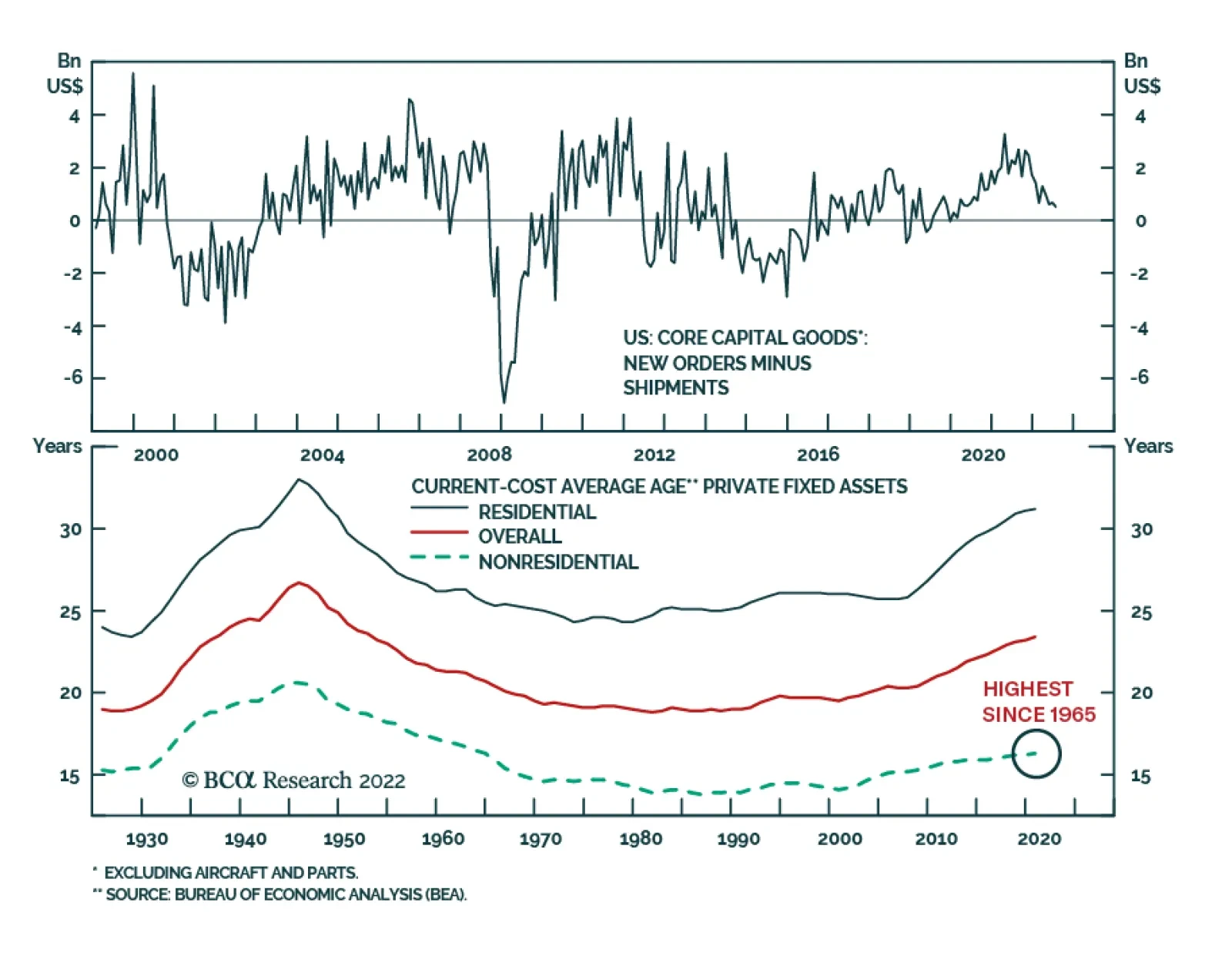
On the surface, the preliminary headline figure for US durable goods orders in July sent a negative signal about the outlook for business spending. US durable goods orders were unchanged, disappointing expectations of a 0.8% m/m increase. However, the…
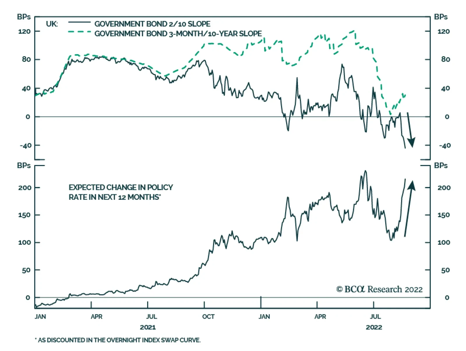
UK Gilts have been selling off sharply since the beginning of August. The yield on the 10-year UK government bond is now over 80bps higher than it was at the start of the month. The move has been even more pronounced at the shorter end of the yield curve.…
Executive Summary Upgrade Euro Area ILBs To Overweight
Upgrade Euro Area ILBs To Overweight
Upgrade Euro Area ILBs To Overweight
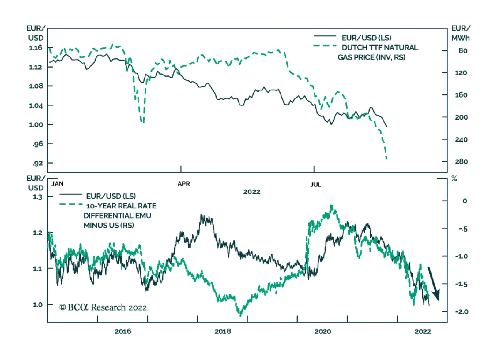
Inflation breakevens have stabilized in the US, where gasoline prices have fallen, but have reaccelerated in the UK and euro area, where natural gas prices have exploded. Inflation breakevens have declined in Canada, potentially due to markets starting to discount a rapid decline in Canadian house price inflation. Our suite of global breakeven models shows that US and Canadian 10-year breakevens are too low, while euro area and UK breakevens are too high. When adjusted for market expectations for the future stance of monetary policies, expressed as the slope of nominal bond yield curves, only the UK stands out with a “conflicted” combination of too-high breakevens and an inverted nominal Gilt curve. Bottom Line: Upgrade inflation-linked bonds to overweight in the euro area (Germany, France, Italy), while downgrading Canadian linkers to underweight. Stay underweight UK linkers, with the Bank of England on course to tip the UK into a deep recession. Maintain a neutral stance on US TIPS, but look to upgrade if the Fed signals a less hawkish path for US monetary policy. Feature Chart 1Intensifying Inflation Worries In Europe
Intensifying Inflation Worries In Europe
Intensifying Inflation Worries In Europe
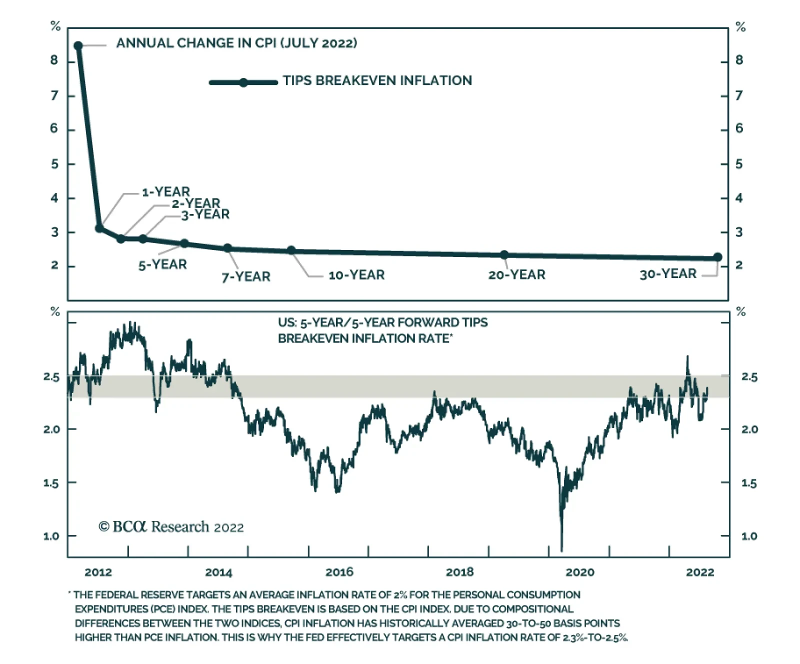
Inflation-linked bonds (ILBs) have played a useful role for fixed income investors looking to protect their portfolios from the pernicious effects of the current era of high inflation. The rising inflation tide had been lifting all global ILB boats. Given the global nature of the brief deflationary shock from the global COVID lockdowns in 2020, and the persistent inflationary shock of the policy-induced recovery from the pandemic, ILB yields – and breakeven spreads versus nominal bonds – have tended to be positively correlated between countries. Now, some interesting divergences have started to appear between market-based inflation expectations (ILB breakevens or CPI swaps) at the country level. Most notably, inflation expectations have been climbing in the euro area and UK, while staying more stable – below the 2022 peak - in the US (Chart 1). In smaller ILB markets like Canada and Australia, breakevens have rolled over and remain at levels consistent with central bank inflation targets even in the fact of high realized inflation. Amid signs of easing inflation pressures from the commodity and traded goods spaces, and with global central banks now in full-blown tightening cycles to try and rein in overshooting inflation, ILB markets are likely to continue being less correlated. Being selective with ILB allocations at the country level, both on the long and short side of the market, will provide better relative return opportunities for bond investors over the next 6-12 months. To assess where those ILB opportunities lie within the developed market universe, we must first go over what is happening with various measures of inflation expectations in each country. A Country-By-Country Tour Of The Recent Dynamics Of Inflation Expectations US Chart 2Lower Gas Prices, Lower US Inflation Expectations
Lower Gas Prices, Lower US Inflation Expectations
Lower Gas Prices, Lower US Inflation Expectations
In the US, the correlation with inflation expectations and gasoline prices remains quite strong (Chart 2). That has been the case when gas prices were soaring, but the correlation works in both directions. The US national gasoline price has fallen by 22% since the peak on June 13, according to the American Automobile Association. Lower gas prices have helped ease consumer inflation expectations. The July reading of the New York Fed’s Survey of Consumer Expectations showed a dip in the 1-year-ahead inflation expectation to 6.2% from 6.8% in June. The 5-year-ahead inflation expectation, which was introduced to the New York Fed survey back in January, fell sharply in July to 2.3% from 2.8% in June (and from a peak of 3% back in March). The fall in US survey-based inflation is also mirrored in lower TIPS breakevens. The 10-year TIPS breakeven fell from 2.76% at the peak of the national gasoline price in mid-June to a low of 2.29% on July 7. The 10-year breakeven has since recovered to 2.58%, but is still below the levels at the time of the peak in gas prices – and considerably lower than the cyclical peak of 3.02% reached in April. The 2-year TIPS breakeven has fallen even more, down from 4.93% to 2.87% since the April peak. UK Chart 3A Historic Energy Price Shock In The UK
A Historic Energy Price Shock In The UK
A Historic Energy Price Shock In The UK
The UK inflation story has been heavily focused on the historic surge in energy prices. UK headline CPI inflation reached double-digit territory in July, climbing to 10.1% on a year-over-year basis, with the energy component of the CPI rising by a staggering 58%. Within that energy component, natural gas prices have been a huge driver, with the gas component of the CPI index up 96% year-over-year in July (Chart 3). Yet despite the relentless climb in energy prices, and the well-publicized “cost of living crisis” with high inflation rates in many non-energy sectors of the UK economy, survey-based measures of UK inflation expectations have stopped rising. The medium-term (5-10 years ahead) inflation expectation from the Citigroup/YouGov survey of UK consumers fell to 3.8% in July, down from the 4.4% peak reached back in March. Even shorter-term inflation expectations have stabilized in the face of rising energy costs (bottom panel). The dip in survey-based inflation expectations as of the July surveys may only be that – a dip – with the 10-year breakeven rate on index-linked Gilts having climbed from 3.8% to 4.2% so far in August. It’s also possible that the household inflation surveys are picking up the impact from the recent slowing of global goods price inflation (and easing global supply chain disruptions). More likely, in our view, UK households are starting to factor in the impact of BoE monetary tightening and an imminent UK recession – one that the BoE is now forecasting – on future inflation. Euro Area Chart 4European Inflation Expectations On The Rise
European Inflation Expectations On The Rise
European Inflation Expectations On The Rise
In the euro area, inflation expectations are finally responding to the steady climb in realized inflation evident across the region. Headline CPI inflation in the region climbed to 8.9% in July, the highest reading since the inception of the euro in 1999. The inflation has been concentrated in a few sectors, with four percentage points of that 8.9% coming from energy prices and another two percentage points coming from food, tobacco and alcohol. Core inflation (excluding food and energy) was 4.0% in July, less alarming than the headline number but still double the ECB’s inflation target of 2%. The ECB now produces its own survey of consumer inflation expectations, which it has been conducting without publishing the results since April 2020. The ECB started publishing the survey this month, as part of a broader Consumer Expectations Survey that also asks questions on topics like future economic growth and the health of labor markets. The most recent survey in June showed that 1-year-ahead inflation expectations were 5%, and 3-year-ahead were 2.8% (Chart 4). Both measures have risen sharply since February – the month before the Russian invasion of Ukraine that triggered the spike in oil and European natural gas prices – when the 1-year-ahead and 3-year-ahead measures were 3.2% and 2.1%, respectively. Euro area market-based inflation expectations are a little more subdued than those from the ECB’s consumer survey. The 5-year breakeven inflation rate on German ILBs is now at 3.4%, while the 10-year breakeven is at 2.5%. A similar message comes from European inflation swaps, with the 5-year measure at 3.4% and the 10-year measure at 2.8%. Canada Chart 5A Housing-Driven Peak In Canadian Inflation Expectations?
A Housing-Driven Peak In Canadian Inflation Expectations?
A Housing-Driven Peak In Canadian Inflation Expectations?
In Canada, realized inflation is still elevated, but may be peaking. Headline CPI inflation was 7.6% in July, down from 8.1% in June, although this came almost entirely from lower energy inflation. Measures of underlying inflation produced by the Bank of Canada (BoC) also stabilized in July, with the trimmed CPI inflation measure ticking down from 5.4% from 5.5% in June (Chart 5). The latest read on survey-based inflation expectations from the BoC’s quarterly Consumer Expectations Survey for Q2/2022 showed a pickup in the 1-year-ahead measure (from 5.1% in Q1 to 6.8%), 2-year-ahead measure (from 4.6% in Q1 to 5%) and 5-year-ahead measure (from 3.2% to 4%). All of those measures are well above the latest readings on market-based inflation expectations from Canadian ILBs, a.k.a. Real Return Bonds, with the 5-year breakeven at 2.2% and 10-year breakeven at 2.1%. Market liquidity is always a factor in the relatively small Canadian Real Return Bond market, yet it is somewhat surprising that breakevens are so low compared with realized and survey-based inflation. The aggressive tightening so far by the BoC, including a whopping 100bp rate hike last month and more expected over the next year, may be playing a role in dampening inflation breakevens – especially with the BoC’s tightening already having an impact on the Canadian housing market. National house price inflation, which tends to lead overall headline CPI inflation by around one year, was 14.2% in July, down from the 2022 peak of 18.8% (top panel). Australia Chart 6Inflation Expectations Remain Moderate In Australia & Japan
Inflation Expectations Remain Moderate In Australia & Japan
Inflation Expectations Remain Moderate In Australia & Japan
In Australia, headline CPI inflation reached 6.1% in Q2/2022, up from 5.1% in Q1/2022, while the median inflation rate was 4.2%. While energy costs were a big contributor to the rise in overall inflation, the pickup was fairly broad-based with notable increases in the inflation rates related to housing (both house prices and furniture prices). Survey-based measures of inflation expectations in Australia focus on more shorter time horizons, thus they are highly correlated to current realized inflation. On that note, the Melbourne University measure of 1-year-ahead consumer inflation expectations soared from 4.9% in Q1/2022 to 6.2% in Q2/2022, while the early read on Q3/2022 2-year-ahead inflation expectations from the Union Officials survey rose to 4.1% from 3.5% in the previous quarter (Chart 6). Market-based inflation expectations are relatively subdued given the high readings of realized inflation and shorter-term survey-based inflation expectations. The 10-year Australian ILB breakeven is now at 1.9%, while the 5-year/5-year forward CPI swap rate is at 2.4%. The aggressive RBA tightening in 2022, with the Cash Rate having increased 175bps over the last four policy meetings, may be playing a role in holding down ILB breakevens. The relatively moderate pace of wage gains in Australia, with the Wage Price Index climbing 2.6% year-over-year in Q2, may also be weighing on ILB breakevens (middle panel). Japan There is not much exciting to say on the inflation front in Japan. The core (excluding fresh food) CPI inflation rate targeted by the Bank of Japan (BoJ) did hit a 7-year of 2.4% in July, but the core CPI measure more in line with international standards (excluding fresh food and energy) was only 1.2% in July (bottom panel). That was the strongest reading since 2015 but still well below the BoJ’s 2% inflation target. Survey-based consumer inflation expectations from the BoJ’s Opinion Survey showed a noticeable increase in Q2/2022, with the 5-year-ahead measure rising to 5% from 3% in Q1. This is obviously well above realized Japanese inflation, although the same survey showed that Japanese consumers believed that the current inflation rate was also 5%. Market-based Japanese inflation expectations are well below the BoJ survey-based measure, but in line with realized core inflation with the 2-year and 10-year CPI swap rates at 1.22% and 0.9%, respectively. The Message From Our Inflation Breakeven Valuation Models Chart 7A Diminished Case For Overweighting Inflation-Linked Bonds
A Diminished Case For Overweighting Inflation-Linked Bonds
A Diminished Case For Overweighting Inflation-Linked Bonds
From an overall global perspective, the case for favoring ILBs versus nominal government bonds across all countries is less intriguing today than was the case in 2021 and early 2022 (Chart 7). Commodity price inflation is slowing rapidly alongside decelerating global growth. This is true both for oil and especially for non-oil commodities, with the CRB Raw Industrials index now falling on a year-over-year basis (middle panel). Supply chain disruptions on goods prices are easing, which is evident in lower rates of goods inflation in the US and other countries. Given the divergences evident between realized inflation, expected inflation and monetary policy outlook outlined in our tour of global inflation expectations, there may be better opportunities to selectively allocate to ILBs on a country-by-country basis. One tool to help us identify such opportunities is our suite of inflation breakeven fair value models. The models are all constructed in a similar fashion, determining the fair value of 10-year ILB breakevens as a function of the same two factors for each country: The underlying trend in realized inflation, defined as the five-year moving average of headline CPI inflation. This forms the medium-term “anchor” for breakevens. The year-over-year percentage change in the Brent oil price, denominated in local currency terms for each country. This attempts to capture cyclical trends around that medium-term anchor based on movements in oil and currencies. We have breakeven fair value models for eight developed market countries, which are shown in the next four pages of this report. The list of countries includes the US (Chart 8), the UK (Chart 9), France (Chart 10), Germany (Chart 11), Italy (Chart 12), Canada (Chart 13), Australia (Chart 14) and Japan (Chart 15). Chart 8Our US 10-Year Inflation Breakeven Model
Our US 10-Year Inflation Breakeven Model
Our US 10-Year Inflation Breakeven Model
Chart 9Our UK 10-Year Inflation Breakeven Model
Our UK 10-Year Inflation Breakeven Model
Our UK 10-Year Inflation Breakeven Model
Chart 10Our France 10-Year Inflation Breakeven Model
Our France 10-Year Inflation Breakeven Model
Our France 10-Year Inflation Breakeven Model
Chart 11Our Germany 10-Year Inflation Breakeven Model
Our Germany 10-Year Inflation Breakeven Model
Our Germany 10-Year Inflation Breakeven Model
Chart 12Our Italy 10-Year Inflation Breakeven Model
Our Italy 10-Year Inflation Breakeven Model
Our Italy 10-Year Inflation Breakeven Model
Chart 13Our Canada 10-Year Inflation Breakeven Model
Our Canada 10-Year Inflation Breakeven Model
Our Canada 10-Year Inflation Breakeven Model
Chart 14Our Australia 10-Year Inflation Breakeven Model
Our Australia 10-Year Inflation Breakeven Model
Our Australia 10-Year Inflation Breakeven Model
Chart 15Our Japan 10-Year Inflation Breakeven Model
Our Japan 10-Year Inflation Breakeven Model
Our Japan 10-Year Inflation Breakeven Model
Full disclosure: we decided last year to de-emphasize our breakeven fair value models after the 2020 COVID recession and, more importantly, the sharp global economic recovery in 2021 from the pandemic shock. The rapid acceleration of oil prices – up 2-3 times in all countries - triggered by that recovery created some wild swings in the estimated breakeven fair value. Today, with oil inflation at more “normal” levels below 100%, we have greater confidence in using the models once again in our strategic thinking on ILBs. The broad conclusions from the models are the following: 10-year inflation breakevens are too low in the US, Canada and Germany 10-year inflation breakevens are too high in the UK and Italy 10-year inflation breakevens are fairly valued in France, Japan and Australia. Taken at face value, our models would suggest overweighting ILBs in the US, Canada and Germany and underweighting ILBs in the UK (and staying neutral on France, Japan and Australia) as part of a new regional ILB diversification strategy. However, there is an additional element to consider when assessing the attractiveness of inflation breakevens at the macro level – the expected stance of monetary policy. ILB inflation breakevens often represent a market-based “report card” on the appropriateness of a central bank’s monetary policy. If monetary settings are deemed to be overly stimulative, the markets will price in higher expected inflation and wider breakevens. The opposite holds true if policy is deemed to be too restrictive, leading to reduced expected inflation and narrower breakevens. Thus, any regional ILB allocation strategy should not only use fair value assessments, but also a monetary policy “filter”. In Chart 16, we show a scatter graph plotting the latest deviations from fair value of 10-year breakevens from our eight country fair value models on the x-axis, and the cumulative amount of expected interest rate increases discounted in overnight index swap (OIS) curves for each country on the y-axis. For the latter, we define this as the peak in rates discounted in 2023 (which is the case for all the countries) minus the trough in policy rates at the start of the current monetary tightening cycle (which is near 0% for all the countries). Chart 16No Clear Link Between Rate Hikes & Breakeven Valuations
A Regional Diversification Strategy For Inflation-Linked Bonds
A Regional Diversification Strategy For Inflation-Linked Bonds
The idea behind the chart is that inflation breakeven valuations should be inversely correlated to the amount of monetary tightening expected by markets. Too many rate hikes would result in markets discounting lower breakevens, and vice versa. However, there is no reliable relationship evident in the chart. For example, the OIS curves are discounting roughly similar levels of cumulative tightening in the US, UK, Canada and Australia, yet ILB breakeven valuations are very different between those countries. In Chart 17, we show a slightly different version of that scatter graph, this time plotting the ILB breakeven fair values versus the slope of the 2-year/10-year nominal government bond yield curve for all eight countries. The logic here is that the slope of the yield curve represents the bond market’s assessment of the appropriateness of future monetary policy. When policy is deemed to be too tight – with an expected peak in rates above what the market believes to be the neutral rate – the yield curve will be flat or even inverted, as markets discount slowing growth in the future and, eventually, lower inflation. Chart 17A Stronger Link Between Yield Curves & Breakeven Valuations
A Regional Diversification Strategy For Inflation-Linked Bonds
A Regional Diversification Strategy For Inflation-Linked Bonds
There is a clear positive relationship between yield curve slope and inflation expectations evident in the new chart. This provides some evidence justifying adding a monetary policy filter to a regional ILB allocation strategy. Related Report Global Fixed Income StrategyDovish Central Bank Pivots Will Come Later Than You Think Under this framework, US and Canadian breakevens trading below fair value is consistent with the inverted yield curves in both countries, with markets now discounting a restrictive level of future interest rates that would dampen inflation expectations. The fair value of Australian and Japanese breakevens also appears in line with the slope of the yield curves in those countries. In terms of divergences, the overvaluation of UK breakevens is inconsistent with the inverted nominal Gilt curve, while the three euro area countries should have somewhat higher breakevens (trading more richly to fair value) given the relatively steeper slope of their yield curves. Investment Conclusions Chart 18Upgrade Euro Area ILBs To Overweight
Upgrade Euro Area ILBs To Overweight
Upgrade Euro Area ILBs To Overweight
After surveying our ILB breakeven fair value models, and cross-checking them versus trends in survey-based inflation expectations and our own assessment of future monetary policies, we arrive at the following country allocations within our new regional ILB strategy: Neutral on US TIPS, despite the attractive valuations. However, look to upgrade if the Fed signals a less hawkish path for US monetary policy (not our base case) or if breakevens fall even further below fair value without more deeper US Treasury curve inversion. Underweight UK ILBs. Breakevens are overshooting due to the near-term inflation risk from soaring energy prices – an outcome that will force the BoE to deliver an even tighter monetary policy, with a more deeply inverted yield curve, that will drive the UK into a disinflationary recession. Underweight Canadian ILBs, despite the attractive valuations. Canadian inflation has likely peaked, and the BoC is engineering a disinflationary downturn in the Canadian housing market with aggressive rate hikes that will maintain an inverted yield curve. Overweight German, French and Italian ILBs. The ECB is likely to deliver fewer rate hikes than markets are discounting, keeping the euro area yield curves relatively steep versus the curves of other developed countries. This also provides a better way to play the near-term inflationary upside from overshooting natural gas prices in Europe than overweighting UK ILBs, with the BoE expected to be much more hawkish than the ECB (Chart 18). Neutral Australia and Japan. Underlying inflation momentum is slower than in the other regions, while breakeven valuations are neutral and not out of line with the expected stance of monetary policy. We are incorporating this new regional ILB strategy into our Model Bond Portfolio, which can be seen on pages 18-20. The changes from current allocations involve upgrades to Germany, France and Italy to overweight, and a downgrade of Canada to underweight. Robert Robis, CFA Chief Fixed Income Strategist rrobis@bcaresearch.com GFIS Model Bond Portfolio Recommended Positioning Active Duration Contribution: GFIS Recommended Portfolio Vs. Custom Performance Benchmark
A Regional Diversification Strategy For Inflation-Linked Bonds
A Regional Diversification Strategy For Inflation-Linked Bonds
The GFIS Recommended Portfolio Vs. The Custom Benchmark Index Global Fixed Income - Strategic Recommendations* Cyclical Recommendations (6-18 Months)
A Regional Diversification Strategy For Inflation-Linked Bonds
A Regional Diversification Strategy For Inflation-Linked Bonds
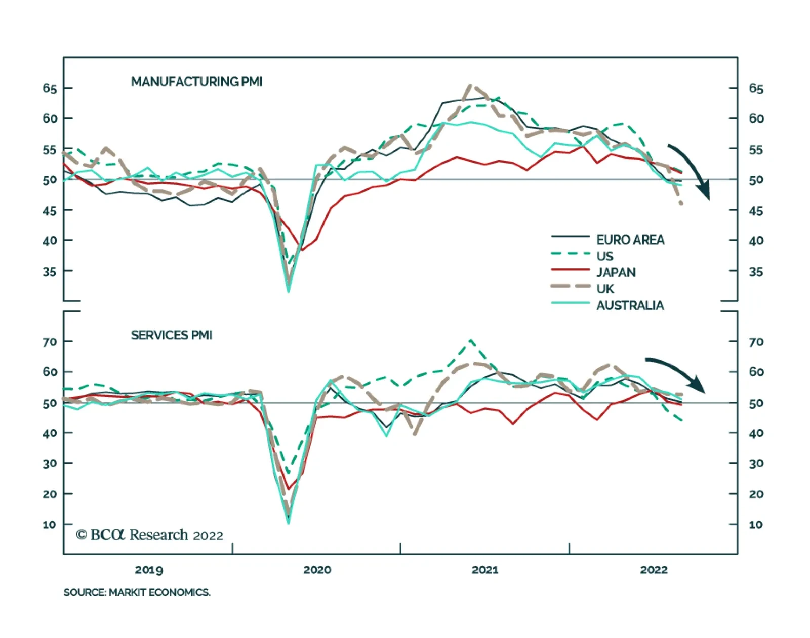
Preliminary estimates point to a broad-based deterioration in DM PMIs in August. Flash manufacturing, services and composite PMIs across the US, Eurozone, Japan, UK and Australia all decreased from July levels. Notably, US services PMI and Eurozone…
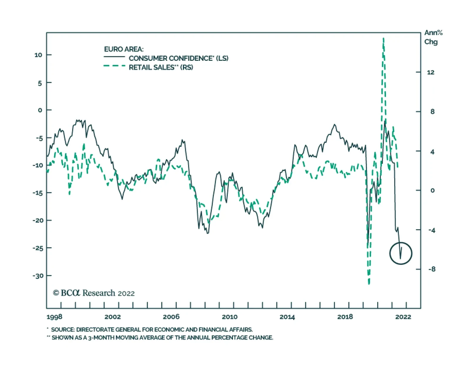
The flash release of the European Commission’s Eurozone consumer confidence in August provides preliminary evidence that sentiment may be in the process of bottoming. It ticked up by 2.1 points to -24.9, surprising expectations of a further deterioration. …
After a brief reprieve since mid-July, EUR/USD has once again broken down over the past week, falling below parity on Monday. The euro’s unrelenting decline over the past year has made it an attractive buy on a valuation basis. Our FX strategists’…
Please note that there will no US Bond Strategy publication next week. Our regular publishing schedule will resume on September 6th with our Portfolio Allocation Summary for September. Executive Summary This report describes a framework for implementing long/short positions in the TIPS market relative to duration-matched nominal Treasuries. The framework is modeled after the Golden Rule of Bond Investing that we use to implement portfolio duration trades. The TIPS Golden Rule states that investors should buy TIPS versus nominal Treasuries when their 12-month headline inflation expectations are above those priced into the market, and vice-versa. We demonstrate a method for forecasting headline CPI inflation and conclude that it will fall into a range of 2.4% to 4.8% during the next 12 months, with risks to the upside. This suggests a high likelihood that headline inflation will exceed current market expectations. The TIPS Golden Rule’s Track Record
The TIPS Golden Rule's Track Record
The TIPS Golden Rule's Track Record
Bottom Line: We see value in TIPS on a 12-month investment horizon but anticipate that an even better entry point to get long TIPS versus nominal Treasuries will emerge during the next couple of months as headline CPI weakens. We recommend a neutral allocation to TIPS for now, though we are looking for a good opportunity to increase exposure. Feature Regular readers will no doubt be familiar with our Golden Rule Of Bond Investing, the framework we use to think about our portfolio duration recommendations. In brief, the Golden Rule states that investors should set their overall bond portfolio duration based on how their own 12-month fed funds rate expectations differ from the expectations that are priced into the market. Our research shows that this investment strategy has a strong historical track record.1 The thing we like most about the Golden Rule framework is that it provides us with a good method for filtering incoming information. Does this new piece of news or economic data change our 12-month rate expectations? If not, then we probably don’t want to assign much weight to it when setting our portfolio duration. In this Special Report we demonstrate that the same Golden Rule logic that we apply to duration trading can also be applied to the TIPS market. Specifically, it can be applied to long/short positions in TIPS versus duration-matched nominal Treasuries. Developing The TIPS Golden Rule Before diving into the TIPS Golden Rule, it’s worth running through the logic that underpins this investment strategy. The logic starts with the Fisher Equation – the well-known formula that relates nominal bond yields to real bond yields. Simply, the Fisher Equation can be stated as follows: Nominal Yield = Real Yield + The Cost Of Inflation Protection In financial market terms, we can re-write the equation as: Nominal Treasury Yield = TIPS Yield + TIPS Breakeven Inflation Rate Two of the three variables in this equation have what we call valuation anchors. The nominal Treasury yield’s valuation is anchored by expectations about the future path for the federal funds rate. Put differently, if you buy a 5-year Treasury note and hold it until maturity, your excess returns versus a position in cash are purely determined by the path of the federal funds rate over that 5-year investment horizon. Similarly, the TIPS breakeven inflation rate’s valuation is anchored by expectations about CPI inflation. If held to maturity, the profits from an inflation protection position (long TIPS/short nominals or short TIPS/long nominals) are purely determined by the path of CPI inflation during the investment horizon. It’s worth noting that, unlike the nominal Treasury yield and the TIPS breakeven inflation rate, the TIPS yield has no independent valuation anchor. Within our framework, the best way to forecast the TIPS yield is to follow a 3-step process: Forecast the nominal yield based on a view about the fed funds rate. Forecast the TIPS breakeven inflation rate based on a view about inflation. Use the Fisher Equation to combine the results from steps 1 and 2 into a forecast for the TIPS yield. As an aside, while our framework relies on viewing the nominal Treasury yield and the TIPS breakeven inflation rate as reflective of expectations for the fed funds rate and CPI inflation respectively, we do not argue that those bond yields can be used to accurately forecast the fed funds rate or CPI inflation. In fact, history tells us that bond markets are usually poor predictors of future outcomes for the fed funds rate and for CPI inflation. Chart 1 shows that there is only a loose correlation (R2 = 22%) between 12-month bond-market implied expectations for the change in the fed funds rate and the actual change in the fed funds rate. Similarly, Chart 2 shows that there is hardly any correlation (R2 = 3%) between market-implied inflation expectations and the 12-month rate of change in headline CPI. Chart 1Market Prices Are A Poor Predictor Of The Fed Funds Rate
The Golden Rule Of TIPS Investing
The Golden Rule Of TIPS Investing
Chart 2Market Prices Are A Poor Predictor Of Inflation
The Golden Rule Of TIPS Investing
The Golden Rule Of TIPS Investing
In other words, it’s more advisable to view the expectations priced into bond markets as a breakeven threshold for trading, not as a tool for forecasting. Stating The TIPS Golden Rule To apply the TIPS Golden Rule, investors should follow these three steps: Calculate market-implied expectations for what headline CPI inflation will be over the next 12 months. This can be done by looking at the 1-year CPI swap rate or the 1-year TIPS breakeven inflation rate.2 Develop an independent forecast for 12-month headline CPI inflation. We demonstrate one method for doing this later in the report.3 Compare your own headline CPI forecast with the forecast that is priced in the market. If your own forecast is higher, then you should go long TIPS/short nominal Treasuries. If your own forecast is lower, then you should go short TIPS/long nominal Treasuries. Testing The TIPS Golden Rule Chart 3 shows the historical track record of the TIPS Golden Rule going back to 2005.4 The top panel shows 12-month excess returns from the Bloomberg Barclays TIPS index relative to a duration-matched position in nominal Treasuries. The bottom panel shows whether inflation surprised market expectations to the upside or to the downside during the investment horizon. We can see that, visually, it looks as though TIPS tend to outperform nominal Treasuries when there is an inflationary surprise and underperform when there is a deflationary surprise. Chart 3The TIPS Golden Rule's Track Record
The TIPS Golden Rule's Track Record
The TIPS Golden Rule's Track Record
Chart 4 shows the same relationship in a little more detail. The 12-month inflation surprise is placed on the x-axis and 12-month TIPS excess returns are on the y-axis. For the TIPS Golden Rule to be useful, we would need to see most of the datapoints in the top-right and bottom-left quadrants of the chart, and indeed this is the case. Chart 412-Month TIPS Excess Returns Vs. Inflation Surprises
The Golden Rule Of TIPS Investing
The Golden Rule Of TIPS Investing
Finally, Table 1 shows the relationship in even more detail. It shows that inflationary surprises coincide with positive TIPS excess returns 73% of the time for an average excess return of 2.6%. It also shows that deflationary surprises coincide with negative TIPS excess returns 80% of the time, for an average excess return of -3.2%. Table 112-Month TIPS Excess Returns* And Inflation Surprises (2005 – Present)
The Golden Rule Of TIPS Investing
The Golden Rule Of TIPS Investing
Please note that all the above return calculations are performed on the overall Bloomberg Barclays TIPS Index relative to a duration-matched position in nominal Treasuries. However, the TIPS Golden Rule also performs well when applied to TIPS of any maturity. The Appendix of this report replicates the above analysis for every point along the TIPS curve and shows that the results are consistently excellent. Applying The TIPS Golden Rule Now that we have stated the TIPS Golden Rule and demonstrated its effectiveness as an investment strategy, it is time to apply it to the current market. To do that, we first determine 1-year market-implied inflation expectations by looking at the 1-year CPI swap rate. As of last Friday’s close, the 1-year CPI swap rate is 3.16%. This means that if we think headline CPI inflation will be above 3.16% during the next 12 months, then we should go long TIPS versus duration-matched nominal Treasuries. If we think headline CPI inflation will come in below 3.16% during the next 12 months, then we should go short TIPS versus duration-matched nominal Treasuries. Next, we must build up our own forecast of headline CPI inflation for the next 12 months. To do this, we follow a bottom-up approach where we split the CPI basket into five components (energy, food, shelter, core goods, and core services ex. shelter) and model each one individually. Energy Inflation (9% Of Headline CPI) Chart 5Modeling Energy Inflation
Modeling Energy Inflation
Modeling Energy Inflation
Energy accounts for roughly 9% of headline CPI, though its often violent price swings mean that this component usually accounts for a much larger percentage of the volatility in headline CPI. In practice, we can accurately model Energy CPI using the prices of retail gasoline, natural gas, and heating oil (Chart 5). To get a 12-month forecast for Energy CPI we therefore need forecasts for the prices of retail gasoline, natural gas, and heating oil. In this analysis, we will consider two possible scenarios for energy prices. First, a benign ‘low oil price’ scenario where we assume that the prices of retail gasoline, natural gas and heating oil follow the paths discounted in their respective futures curves. Second, we consider a ‘high oil price’ scenario that incorporates the view of our Commodity & Energy Strategy service that a drop in Russian oil supply, among other factors, will cause the Brent crude oil price to reach $119 per barrel by the end of this year and average $117 per barrel in 2023.5 To incorporate this outlook into our model, we regress the prices of retail gasoline, natural gas and heating oil on the Brent crude oil price and extrapolate forward using our commodity strategists’ forecasts. The ‘low oil price’ scenario has Energy CPI inflation falling from its current 32.9% level all the way down to -9.9% during the next 12 months. In contrast, our ‘high oil price’ scenario has it falling to just 15.8%. Food Inflation (13% Of Headline CPI) Chart 6Modeling Food Inflation
Modeling Food Inflation
Modeling Food Inflation
Our Food CPI model is based on the cost of fertilizer, agricultural commodity prices and diesel prices. This model has done a reasonably good job explaining trends in Food CPI inflation over time, but the last few months have seen food inflation jump well above the levels suggested by our model (Chart 6). Given that the inputs to our Food CPI model are highly correlated with the oil price, we also apply the ‘low oil price’ and ‘high oil price’ scenarios discussed above to our Food CPI forecast. Using this method, the ‘low oil price’ scenario has Food CPI inflation falling to 3.8% during the next 12 months and the ‘high oil price’ scenario has it coming down to 4.2%. One key risk to these forecasts is that they both assume that the current gap between food inflation and our model’s fair value will close. It’s possible that other factors not included in our model could prevent the gap from closing. We therefore consider our Food CPI forecast to be quite optimistic. Core Goods Inflation (21% Of Headline CPI) Chart 7Modeling Goods Inflation
Modeling Goods Inflation
Modeling Goods Inflation
Core goods inflation, currently running at 6.9%, appears to have already peaked following its post-pandemic surge. We model Core Goods CPI using the New York Fed’s Global Supply Chain Pressure Index, as it is the supply chain constraints that arose during the pandemic that explain the bulk of the movement in core goods prices since that time (Chart 7).6 To forecast Core Goods CPI, we assume that global supply chain constraints continue to ease and that the New York Fed’s index reverts to its pre-pandemic level during the next 12 months. This gives us a forecast for 12-month Core Goods CPI inflation of 0%. Shelter Inflation (32% Of Headline CPI) Chart 8Modeling Shelter Inflation
Modeling Shelter Inflation
Modeling Shelter Inflation
We model shelter inflation, currently running at 5.6%, using the unemployment rate, rental vacancy rate and home prices (Chart 8). Except for the unemployment rate, all our model’s independent variables enter with a lag of at least 12 months. In other words, we wouldn’t expect any near-term change in home prices to impact Shelter CPI for at least a year. To forecast Shelter CPI, we assume that the unemployment rate rises to 4% during the next 12 months. This results in a shelter inflation forecast of 4.7% for the next 12 months. Much like with food inflation, we tend to view this forecast as relatively optimistic as it assumes a large reversion from the current rate of shelter inflation back to our model’s fair value. It’s conceivable that other factors not included in our model, such as rapid wage growth, could prevent this reversion from occurring. Services ex. Shelter Inflation (24% Of Headline CPI) Chart 9Modeling Services Inflation
Modeling Services Inflation
Modeling Services Inflation
This final component of CPI is a bit of a hodgepodge of different service industries that may not have much in common. However, we find that wage growth does a good job of tracking its trends (Chart 9). We therefore model Services ex. Shelter CPI using the Employment Cost Index, which enters our model with a 10 month lag. To forecast Services ex. Shelter CPI, we assume that the Employment Cost Index holds steady at its current growth rate. This gives us a Services ex. Shelter CPI inflation forecast of 5.5% for the next 12 months. Combining Our Bottom-Up Inflation Forecasts & Investment Conclusions Combining our bottom-up forecasts, we calculate a 12-month headline CPI inflation rate of 2.4% for the ‘low oil price’ scenario and a rate of 4.8% for the ‘high oil price’ scenario. For core CPI inflation, we calculate a 12-month forecast of 3.6%. Given the optimistic assumptions that we incorporated into our forecasts, particularly the large reversions of food and shelter inflation back to our estimated fair value levels, we view the risks to our forecasts as heavily tilted to the upside. We also acknowledge that the re-normalization of global supply chains may not proceed as smoothly as the scenario that is baked into our forecasts. Any hiccup in that process would cause our goods inflation forecast to be too low. Chart 10Inflation Forecasts
Inflation Forecasts
Inflation Forecasts
Chart 10 shows our 12-month headline and core CPI forecasts alongside the market-implied forecast from the CPI swap curve, currently 3.16%. Notice that the market-implied inflation forecast is much closer to the bottom-end of our range of headline CPI estimates, and we have already acknowledged that a lot of things will have to go right for our estimates to pan out. In other words, we see a high likelihood that 12-month headline CPI will be above 3.16% for the next 12 months which, according to our TIPS Golden Rule, tells us that we should go long TIPS versus duration-matched nominal Treasuries. While we acknowledge that there is likely some value in going long TIPS versus nominal Treasuries today, we are inclined to maintain our recommended neutral allocation to TIPS versus nominals for now. Given the recent drop in oil prices, we anticipate further weakness in headline inflation during the next couple of months. This could push TIPS breakeven inflation rates even lower in the near term, creating even more value. The bottom line is that we see attractive value in TIPS versus nominal Treasuries on a 12-month investment horizon. While we maintain a neutral allocation to TIPS for now, we anticipate turning more bullish in the near future, hopefully from a better entry point after one or two more weak CPI prints. Appendix Chart A112-Month TIPS Excess Returns Vs. Inflation Surprises (1-3 Year Maturities)
The Golden Rule Of TIPS Investing
The Golden Rule Of TIPS Investing
Table A112-Month TIPS Excess Returns* And Inflation Surprises (1-3 Year Maturities)
The Golden Rule Of TIPS Investing
The Golden Rule Of TIPS Investing
Chart A212-Month TIPS Excess Returns Vs. Inflation Surprises (3-5 Year Maturities)
The Golden Rule Of TIPS Investing
The Golden Rule Of TIPS Investing
Table A212-Month TIPS Excess Returns* And Inflation Surprises (3-5 Year Maturities)
The Golden Rule Of TIPS Investing
The Golden Rule Of TIPS Investing
Chart A312-Month TIPS Excess Returns Vs. Inflation Surprises (5-7 Year Maturities)
The Golden Rule Of TIPS Investing
The Golden Rule Of TIPS Investing
Table A312-Month TIPS Excess Returns* And Inflation Surprises (5-7 Year Maturities)
The Golden Rule Of TIPS Investing
The Golden Rule Of TIPS Investing
Chart A412-Month TIPS Excess Returns Vs. Inflation Surprises (7-10 Year Maturities)
The Golden Rule Of TIPS Investing
The Golden Rule Of TIPS Investing
Table A412-Month TIPS Excess Returns* And Inflation Surprises (7-10 Year Maturities)
The Golden Rule Of TIPS Investing
The Golden Rule Of TIPS Investing
Chart A512-Month TIPS Excess Returns Vs. Inflation Surprises (10-15 Year Maturities)
The Golden Rule Of TIPS Investing
The Golden Rule Of TIPS Investing
Table A512-Month TIPS Excess Returns* And Inflation Surprises (10-15 Year Maturities)
The Golden Rule Of TIPS Investing
The Golden Rule Of TIPS Investing
Chart A612-Month TIPS Excess Returns Vs. Inflation Surprises (15+ Year Maturities)
The Golden Rule Of TIPS Investing
The Golden Rule Of TIPS Investing
Table A612-Month TIPS Excess Returns* And Inflation Surprises (15+ Year Maturities)
The Golden Rule Of TIPS Investing
The Golden Rule Of TIPS Investing
Ryan Swift US Bond Strategist rswift@bcaresearch.com Robert Timper Research Analyst robert.timper@bcaresearch.com Footnotes 1 Please see US Bond Strategy Special Report, “The Golden Rule Of Bond Investing”, dated July 24, 2018. 2 In this report we use the 1-year CPI swap rate because it is easier to access. 3 To make the TIPS Golden Rule easy to implement, we use seasonally adjusted headline CPI for all our calculations even though TIPS are technically linked to the non-seasonally adjusted index. We also ignore the fact that TIPS coupons adjust to CPI releases with a lag. Our analysis shows that the rule works very well even without incorporating these complications. 4 CPI swap rates are only available from 2004 onwards, so this is the largest historical sample we can use. 5 Please see Commodity & Energy Strategy Weekly Report, “EU Russian Oil Embargoes, Higher Prices”, dated August 18, 2022. 6 For more details on the Global Supply Chain Pressure Index: https://www.newyorkfed.org/research/policy/gscpi#/overview Recommended Portfolio Specification Other Recommendations Treasury Index Returns Spread Product Returns
Although the BCA house view calls for a neutral equity allocation on a cyclical 12-month investment horizon, some of our more optimistic colleagues remain tactically overweight. Specifically, our Global Investment strategists have highlighted three key…
Executive Summary The Fed Versus The Market
The Fed Versus The Market
The Fed Versus The Market
In today’s report, we summarize the arguments of bulls and bears to examine the possible longevity of the rally. The Bulls’ view is centered around several key themes: Inflation has turned. The Fed is less hawkish than initially assumed, and Jay Powell is not Paul Volcker. The economy is resilient, and consumers are spending. Corporate earnings will surprise on the upside thanks to consumer strength. Meanwhile, the bears argue that: Growth is slowing and a soft landing is elusive, which will lead to earnings disappointment. Valuations and Technicals are no longer attractive – the best part of the rally is likely over, and risk-reward is skewed to the downside. Inflation is embedded and broad-based and it will take many months to reach the level that is palatable to the Fed. Bottom Line: The rally was expected, but its force and durability took us by surprise. Now, after a strong rebound, risks are skewed to the downside and the markets are fragile, but the rally may continue. We offer our take on what can bring this rally to a halt, and the “danger” signs investors need to be on the lookout for. Feature The fast and furious rally off the June 16 lows has taken many investors by surprise. Over the past two months, the S&P 500 has rebounded by 17%, the NASDAQ is up 22%, while Growth has outperformed Value by 9%. Thematic small-cap growth ETFs have fared even better (Chart 1) with Cathie Wood’s ARKG and ARKK up nearly 50%. The Technology and Consumer Discretionary sectors are up 23% and 28% respectively, while Energy and Materials are relatively flat, showcasing a rotation away from the inflation winners to losers. In this week’s report, we will “dissect” the rally and its key drivers to better understand what can bring this rally to a halt. We will also summarize the arguments of the bulls and present our “bearish” rebuttal to some of the assumptions. Sneak Preview: After the powerful rebound, the market is fragile, and risks are skewed to the downside. By summarizing the arguments of bulls and bears, we are offering our take on what can bring this rally to a halt, i.e., hawkish Fed speeches, disappointing inflation readings, rising rates, and bad earnings. However, a positive surprise along each of these dimensions may also result in the next leg up. Chart 1ETF Universe Overview
What Can Bring This Rally To A Halt?
What Can Bring This Rally To A Halt?
Anatomy Of The Rally To understand what fuels the rally, we need to understand what its key catalysts are. Oversold: First and foremost, in mid-June, US equities were severely oversold – the BCA Capitulation Indicator hit levels last seen in the spring of 2020 (Chart 2). The BoA institutional survey has also reported an extreme level of bearishness. Pull back in the price of energy: This created fertile ground for a rebound, but the catalyst came from the turn in commodities and energy prices. Extreme pessimism about global growth after the Fed’s aggressive response to a disappointing inflation print has triggered a sell-off in oil and metals. Since mid-June, the GSCI Commodities and the GSCI Energy index are in a bear market downtrend, 21% and 25% off their peaks. Inflation moderating: This disinflationary development has unleashed a positive reinforcement loop: Lower energy prices led to a turn in the CPI print. And many still believe that, after all, inflation is transitory: With supply disruptions clearing and prices of energy and commodities turning, inflation will dissipate just as fast as it arrived. We know this because inflation breakevens are currently at levels last seen a year ago (Chart 3). Chart 2Capitulated
Capitulated
Capitulated
Chart 3Cooling Off : Back To 2021
Cooling Off : Back to 2021
Cooling Off : Back to 2021
Gentler Fed: That is when the market decided that easing price pressures in concert with slowing growth would compel the Fed to pursue a shallower and shorter path of interest rate increases than initially expected – rate increases derived from OIS started to undershoot the “dot plot” (Chart 4). Effectively, the bond market started to forecast that the Fed will end the year at 3.5% and ease as soon as early 2023. In other words, the Fed is nearing the end of the hiking cycle. Naturally, the long end of the Treasury curve has pulled back to April levels, despite a much higher Fed rate. One way or another, yields have stabilized. Lower rates are a boon for equities: As a long-duration asset, equity valuations are inversely correlated with long yields (Chart 5). A better-than-expected Q2 earnings season was the icing on the cake. Chart 4The Market Expects Cuts As Soon As Early 2023
The Market Expects Cuts As Soon As Early 2023
The Market Expects Cuts As Soon As Early 2023
Chart 5Falling Yields Propelled Equities Higher
Falling Yields Propelled Equities Higher
Falling Yields Propelled Equities Higher
Was The Rally Surprising? The rally itself did not surprise us – after all, we did expect the market to turn on a dime at the earliest whiff of falling inflation (Chart 6). Admittedly, we were taken aback by its strength and longevity. With inflation turning, we also expected a change in leadership from the Energy and Materials sectors to Technology and Consumer Discretionary (Chart 7). We also predicted back in January in our “Are We There Yet?!” report that, based on the previous hiking cycles, Tech would rebound roughly three months after the first rate hike (Chart 8), which was taking us to June. Chart 6When Inflation Turns, Equities Rebound
What Can Bring This Rally To A Halt?
What Can Bring This Rally To A Halt?
Chart 7Turn in Inflation Triggers A Change In Sector Leadership
What Can Bring This Rally To A Halt?
What Can Bring This Rally To A Halt?
Chart 8A Closer Look At Technology
What Can Bring This Rally To A Halt?
What Can Bring This Rally To A Halt?
In early July, we upgraded Growth to overweight as an asset that would benefit from an anticipated turn in CPI, rate stabilization, and slowing growth (Chart 9). We have also reaffirmed our overweight in Software and Services as a way to play Growth on a sector level. We have downgraded Energy to underweight to reduce exposure to Value. Chart 9Growth And Quality Lead Markets Higher When Inflation Abates
What Can Bring This Rally To A Halt?
What Can Bring This Rally To A Halt?
What The Bulls Think Let’s summarize what the bulls think are the catalysts for the next leg up: Inflation has turned. Looking for further signs that inflation is easing. The Fed is less hawkish than initially assumed, and Jay Powell is not Paul Volcker. Looking for signs that the Fed is getting closer to the end of the hiking cycle. So far, the economy is resilient, and consumers are spending – excess savings and excess demand for labor will soften the blow. Looking for signs that the recession can be avoided. Corporate earnings will surprise on the upside thanks to consumer strength. In the next section, I will juxtapose these optimistic expectations with those of a bear, i.e., of yours truly. A full disclosure – I am not a perma-bear but even eight weeks into the best recovery rally ever, I can’t shake off my pessimism. After all, I am used to the markets going up on injections of liquidity and expect them to shudder when liquidity is mopped out of the system. What The Bears Think, Or A Litany Of Worries Inflation is embedded and broad-based Broad-based: While headline inflation is turning, mostly thanks to prices of energy and materials, it will take a long time for core inflation to revert to the desired 2% as it is broad-based. This is evident from trimmed and median CPI metrics, which continue their ascent. Inflation has also spilled into sticky service items, such as rent (Chart 10). Wage-price spiral: Then there is that pesky wage-price spiral that is manifesting itself in soaring labor costs (Chart 11), which companies pass on to their customers. In the meantime, productivity is falling, and unit labor costs are increasing at 9.5% per year, a rate of growth last seen in 1980s (Chart 12). Demand for labor still exceeds supply with 1.8 job openings for every job seeker, and much more tightening is required to bring supply and demand into balance. Chart 10Entrenched?
Entrenched?
Entrenched?
Chart 11Wage-price Spiral
Wage-price Spiral
Wage-price Spiral
Chart 12ULC Soaring
ULC Soaring
ULC Soaring
Wages and service inflation are more important to structural inflation than energy. Rent and its equivalents constitute 30% of the CPI basket, while wages are roughly 50% of corporate sales and by far the largest component of the cost structure. Inflation is embedded and broad-based and it will take many months to reach the level that is palatable to the Fed. What Does The Fed Think? Fed minutes: Fortunately, we don’t need to guess. The Fed minutes state that "participants agreed that there was little evidence to date that inflation pressures were subsiding" and that inflation “would likely stay uncomfortably high for some time.” Further, “though some inflation reduction might come through improving global supply chains or drops in the prices of fuel and other commodities … Participants emphasized that a slowing in aggregate demand would play an important role in reducing inflation pressures," the minutes said. The Fed minutes state that in moving expeditiously to neutral and then into restrictive territory, “the Committee was acting with resolve to lower inflation to 2% and anchor inflation expectations at levels consistent with that longer-run goal.” In its previous communications, the Fed emphasized that its commitment to a 2% target is unconditional. Is powell more like burns or volcker? In addition, there is an ongoing debate between bulls and bears on the character of the Fed – is Jay Powell a strong-willed hawk like Paul Volker, or more of a waverer like Arthur Burns, who presided over the relentless march of inflation in the seventies? We think that the Chairman can channel Paul Volcker. After all, the Fed has surprised investors by acting swiftly and decisively. Back in March, the Fed dot plot indicated that by the end of the year, the target rate will reach a mere 1.75%. However, we hit a 2.25%-2.50% rate range as soon as July. Jay Powell is concerned about his legacy: He would not want to be remembered as a Chair who mishandled inflation by keeping rates too low despite historically low unemployment and resilient consumers whose accounts are padded with excess post-pandemic savings. The Fed is more hawkish than what the majority of market participants, unscathed by the inflation of the seventies and eighties, believe. The Fed dot plot, to which the Chairman referred on multiple occasions, projects a Fed funds rate of 4% at year-end and of 4.5-5.0% next year (Chart 13). Meanwhile, Fed funds futures are only pricing a rate of about 3.4% for December 2022, even after the hawkish talk from both ex-dove Kashkari and a hawk Bullard (3.75%-4.0% by year-end and 4.4% by the end of 2023). Further, the Fed itself states in its minutes that rates would have to reach a "sufficiently restrictive level" and remain there for "some time" to control inflation that was proving far more persistent than anticipated. The Chicago Fed President Charles Evans has also affirmed that the Fed is definitely not cutting rates in March 2023. Chart 13The Fed Versus The Market
The Fed Versus The Market
The Fed Versus The Market
Doves latch on to comments from the meeting that the Fed will be data-driven, and that it is concerned about overtightening. To us, these are just the musings of the “responsible grown-ups.” Quantitative Tightening: Now let’s not forget another leg of the stool – Quantitative Tightening. QT has been very tame so far and, since the program commenced, the size of the Fed’s balance sheet, $8.9 trillion, has barely budged. In September, the Fed is scheduled to step up QT to a maximum pace of $95 billion from $47.5 billion— running off up to $60 billion in Treasuries, and $35 billion of mortgage securities. Shortages of securities available for run-off due to a dearth of refinancing may trigger a shift to outright selling, further tightening financial conditions. Equities are at odds with the Fed: Last, but not least, equity markets are on a collision course with the Fed. Since June, financial conditions have eased as opposed to tightened, making the Fed’s job so much harder (Chart 14). Chart 14The Rally Eased Financial Conditions
The Rally Eased Financial Conditions
The Rally Eased Financial Conditions
The Fed may prove to be more hawkish than in the past as it is on a quest to combat inflation and takes its mission very seriously. “Don’t fight the Fed” the adage holds. Economic Growth Is Slowing The BCA Business Cycle Indicator signals that economic growth is slowing (Chart 15), which is also evident from a host of economic data releases, ranging from GDP growth to business surveys to housing data. One of the few data series that has defied gravity so far is the jobs report, but the job creation rate is a coincidental indicator at best, and a lagging one at worst. Jobs are usually lost after the start of a recession (Chart 16). Chart 15Economy Is Slowing
Economy Is Slowing
Economy Is Slowing
Chart 16Unemployment Never "Just Ticks Up"
Unemployment Never "Just Ticks Up"
Unemployment Never "Just Ticks Up"
Can consumers save the day? After all, $2.2 trillion in excess savings should help to handle the pressures of negative real wage growth and income growth that is below trend. Yes and no. Gasoline savings can certainly support increases in discretionary spending, all else equal. As for excess savings – adding this money back into the economy may ignite another bout of inflation, working against the Fed, and triggering more rate increases. Many clients ask us if we anticipate a recession. Broadly speaking we do, as the Fed has an arduous task ahead of it in balancing the supply and demand of labor. However, we do not expect a recession in 2022 or even early 2023. Can the Fed succeed by only reducing excess job openings from 1.8 to 1, thus avoiding a rise in unemployment? This is possible, but the probability of such an outcome is low as unemployment never “just ticks up” (Chart 16). However, what the market is pricing is also important. At the moment, the rally shows that it considers the current growth slowdown just a growth scare to be shrugged off. Will there be more disappointments? We think so, as the US economy is facing multiple headwinds from slowing demand for exports due to geopolitical turbulence and payback of overstimulated consumer demand at home. And it is not a recession per se, but a growth disappointment, that may take equities on the next leg down. Growth is slowing and a soft landing is illusive. Earnings Growth Will Continue Its March Towards Zero We believe that earnings growth will continue to slow into year-end – flagging consumer demand at home and abroad, a strong dollar, and soaring unit labor costs that can no longer be fully passed on to stretched consumers, as corporate pricing power is decelerating. Even in Q2-2022, ex-Energy EPS growth is already negative at -1.5%, with Consumer Discretionary, Financials, Communications, and Utilities reporting an earnings contraction. As we predicted back in October, the S&P 500 margins are also compressing, currently at 50bps off their peak, with consensus expecting them to lose another two points within the next 12 months as companies are grappling with rising costs (Chart 17). Analysts are finally in a downgrading mode (Chart 18), with growth over the next 12 months now expected to be 7.7% compared to 10% earlier this summer. Analyst downgrades will continue, and an earnings recession is highly probable as early as Q4-2022. Chart 17Profitability Is Under Pressure
Profitability Is Under Pressure
Profitability Is Under Pressure
Chart 18Earnings Are Finally Being Downgraded
Earnings Are Finally Being Downgraded
Earnings Are Finally Being Downgraded
In terms of the durability of the rally – earnings growth disappointment will be enough to cause equities to pull back. Earnings growth is slowing and more disappointments may be in store. Valuations And Technicals The S&P 500 is currently trading at 18x forward earnings, which is nearly a two-point rebound off the market trough of 15.8x. This is roughly where PE NTM was in April when the 10-year yield stood at 2.80%. Therefore, the multiple reverted on the back of falling rates, and the market is fairly valued considering where rates are now. And another factor to consider: Analysts are slashing earnings expectations, and with E in a P/E likely to be downgraded further – the “true” forward multiple is likely higher than it appears. The BCA Valuation Indicator is also flashing “overvalued” (Chart 19). From the equity risk premium standpoint, 3% is low by historical standards (Chart 20). And if we consider Shiller PE, it has come down from an eye-watering 38x to a still elevated 29x. Chart 19Pricey Again?
Pricey Again?
Pricey Again?
Chart 20Equities Are No Longer Cheap By ERP Or Shiller PE Metrics
Equities Are No Longer Cheap By ERP Or Shiller PE Metrics
Equities Are No Longer Cheap By ERP Or Shiller PE Metrics
Therefore, it is hard to call equities cheap at this point. But being generous, we will call them “fairly priced.” Regardless – at these levels of valuations, the best part of the rally is likely over, and risk-reward is no longer favorable. From a technical standpoint, this rally is broad-based with nearly 90% of the S&P 500 industries trading above their 50-day moving average (Chart 21). But according to the BCA Technical Indicator, equities are no longer oversold and have just crossed into neutral territory (Chart 22). Interestingly, once the Technical indicator starts to rise, it usually ascends for a while, making us wary to boldly call an immediate end to this rally. Chart 21Thrusting
Thrusting
Thrusting
Chart 22No Longer Oversold?
No Longer Oversold?
No Longer Oversold?
Valuations and Technicals are no longer attractive – the best part of the rally is likely over and risk-reward is skewed to the downside. Investment Implications Or Can This Rally Continue? Timing the market is hard at best, impossible at worst. After a 17% rise from the bottom, the S&P 500 is no longer cheap or oversold. Buying equities for valuations or technical reasons is too late – risks are skewed to the downside. Our working assumption is that the rally will pause waiting for the new data that will trigger a new leg up or down. Further, as we pointed out in the Fat and Flat report, the current period is reminiscent of the 1980-1982 Volcker era. So far, the market is following this pattern to a T (Chart 23). The problem is that each leg of the up-and-down market may take months. As such, being (eventually) right and principled does not pay off. After all, the economy is not a market. Therefore, until one of the following happens, the music will continue and the markets can keep dancing, which may be for a while. Chart 23Volcker Era Redux
Volcker Era Redux
Volcker Era Redux
The rally will continue until: There is a communication from the Fed re-emphasizing its hawkish stance and determination to get inflation back to 2%. It may be as one of the FOMC member’s speeches broadcast at Jackson Hole. Long-term Treasury yields pick up either because of the Fed’s actions or speeches or because the economy is overheating. Negative inflation surprise – it may come as either a higher-than-expected inflation reading or evidence that inflation is entrenched, such as rising service or rent inflation, soaring wages, a pick-up in the price of oil or commodities, or a growth surprise out of China, to name but a few. Negative earnings surprise – guidance from a number of companies indicating that economic growth is slowing, and earnings will disappoint. A negative economic surprise may be perceived by the market as “bad news is good news.” We recommend the following: Maintain a well-diversified portfolio, with sufficient allocation to both cyclicals and defensives. Increase exposure to Growth sectors, such as Technology. We particularly favor Software and Services as it leverages the pervasive theme of digitization and migration to the cloud. Reduce allocation to Energy and Materials – these sectors tend to underperform when inflation turns. They are also quintessential value sectors. Maintain some allocation to cyclicals – we are overweight the Industrial sector as it leverages a long-term theme of onshoring and automation. We may be upgrading the Consumer Discretionary sector in the near future. We are also overweight Banks and Insurance for portfolio diversification – these sectors benefit from rising rates and positive growth surprise. Markets turn on a dime and it is good to be prepared. Allocate capital to long-term investment themes: Green and Clean and EV, benefiting from the funds allocated by the IRA bill, Cyber Security, and Defense. Bottom Line: The rally was expected, but its force and durability took us by surprise. Now, after a strong rebound, risks are skewed to the downside and the markets are fragile, but the rally may still continue. We offer our take on what can bring this rally to a halt, and the “danger” signs investors need to be on the lookout for. In the meantime, overweight Growth and maintain a well-diversified portfolio. Irene Tunkel Chief Strategist, US Equity Strategy irene.tunkel@bcaresearch.com Recommended Allocation Recommended Allocation: Addendum
What Our Clients Are Asking: The Bear Market 2.0 Webcast Follow Up
What Our Clients Are Asking: The Bear Market 2.0 Webcast Follow Up