Lumber

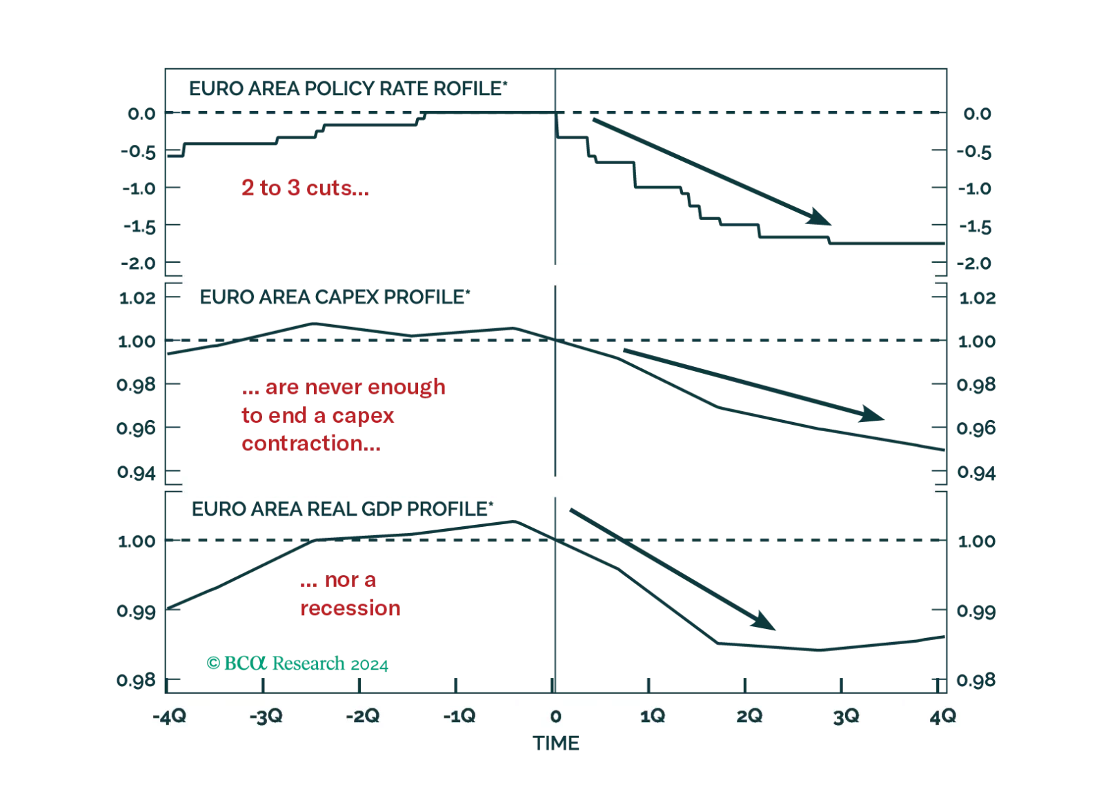
Investors hope that the ECB rate cuts priced into the curve will be sufficient to achieve a soft landing in Europe. History argues against this view, but will this time be different?

Highlights Domestic and foreign supply-side constraints are now exerting a significant effect on the US economy. Consumer prices may increase at a faster pace than we initially expected over the coming 3-4 months, but supply-side constraints are likely to wane later this year and thus do genuinely appear to be transitory. The idea that even a temporary period of high inflation could persist over the longer term has legitimate grounding in macro theory, and is explicitly recognized in the Fed’s inflation framework. But it would necessitate a very large increase in inflation expectations, which have yet to rise to abnormal levels. The baseline for inflation has shifted back closer to the Fed’s target, but deviations above or below target over the coming 12-18 months are likely to be driven by demand-side rather than supply-side factors. The Fed’s checklist for liftoff now entirely depends on employment, and there are compelling arguments in favor of outsized jobs growth in the second half of the year that would move forward the timing of the first rate hike. But the reality for investors is that there is tremendous uncertainty concerning the magnitude of these job gains, given the likelihood of some lasting changes to consumer behavior following the pandemic. Visibility about the employment consequences of these changes will remain very low until investors receive more information about likely urban office footprint and downtown commuter presence, the speed at which international travel will return, and to what degree any pandemic control measures remain in place in the second half of the year. For now, investors should remain cyclically overweight stocks versus bonds, short duration, and invested in other procyclical positions, with an eye to reassess the monetary policy and growth outlook in the late summer / early fall. Feature Chart I-1Investors Have Focused On The April Jobs And Inflation Data Investors Have Focused On The April Jobs And Inflation Data Investors Have Focused On The April Jobs And Inflation Data Investors’ attention in May was focused squarely on two, ostensibly contradictory US data surprises: an extremely disappointing April jobs report, and a surge in consumer prices (Chart I-1). Abstracting from the typically lagging nature of consumer prices, a weak labor market is typically disinflationary / deflationary, not inflationary. But this is only to be expected in a typical environment where demand-side factors are predominantly driving the jobs market and the pricing decisions of firms, and the April data has made it clear that domestic and foreign supply-side constraints are now exerting a significant effect on the US economy, more forcefully than we initially thought. This warrants a further analysis of our prior view that supply-side effects would have a moderate effect on activity and prices this year, which we present below. A Deep Dive Into April’s Employment And Inflation Data Chart I-2 shows the difference between the April monthly gain in US jobs by industry compared with those of March. Almost all US industries saw a slower pace of jobs gains in April than March, but the slowdown was particularly acute in the professional & business services, transportation & warehousing, education & health services, construction, and manufacturing industries. By contrast, leisure & hospitality, the industry with the largest employment gap relative to pre-pandemic levels, saw a faster pace of April job gains relative to March. Chart I-2Breaking Down Disappointing April Payroll Gains June 2021 June 2021 In our view, several facts from the April jobs report characterize the labor market as being in a transition towards a post-pandemic state, but also legitimately impacted by labor supply constraints at the low-skilled and blue-collar levels: Within professional & business services, almost all of the slowdown in monthly job gains occurred within temporary help services. Temp help services is a cyclical employment category over the longer-term, but over short periods of time it can also be negatively correlated with gains in full-time positions. April saw a large decline in the number of employed persons at work part time, suggesting that the slowdown in temp help may reflect a shift back to full-time work. Within transportation & warehousing, the slowdown in jobs was entirely attributed to the couriers and messengers subsector, which includes delivery services. In combination with the acceleration in jobs in the leisure & hospitality sector, this likely reflects a shift away from home food delivery towards in-person restaurant orders and the use of aggressive hiring tactics by restaurant owners (including advertisements of cash bonuses following 90 days of completed work, paid vacations, health insurance, and other perks). The slowdown in jobs growth in the construction & manufacturing industries is likely due to two, separate supply constraints: the negative impact of higher input costs such as lumber, semiconductors, and other raw materials, as well as the disincentivizing effects of supplementary unemployment benefits that appears to be limiting the willingness of lower-wage workers to return to work. Chart I-3April's Rise In Core CPI Was Extreme, Even After Removing Some Outliers April's Rise In Core CPI Was Extreme, Even After Removing Some Outliers April's Rise In Core CPI Was Extreme, Even After Removing Some Outliers On the inflation front, Chart I-3 highlights that the April surge in core consumer prices did not just occur because of year-over-year base effects, but because of significant month-over-month increases in prices. Outsized gains in used car prices driven by the impact of the semiconductor shortage on new car production, as well as surging airline fares, did significantly contribute to April’s month-over-month gain, but the dotted line in the chart highlights that the monthly change would still have been extreme relative to history even if these components had increased instead at a 2% annual rate. Taken together, the April employment and inflation data, in conjunction with surveys of US firms as well as the trend in commodity prices, suggest that the labor market and consumer prices are being affected by four separate but related factors: An underlying demand effect, driven by extremely stimulative fiscal & monetary policy as well as economic reopening; A domestic labor shortage Coordination failures and bottlenecks impacting the production of key supply chain components and resource inputs Coordination failures and bottlenecks impacting the logistics of international trade Strong domestic aggregate demand is not likely to wane over the coming 6-12 months, which has been the basis for our view that inflation would rise to modestly above-target levels this year. Given this new evidence of their prominence and impact, it does seem likely that the remaining three supply-side factors will persist for a few more months, suggesting that core inflation may remain quite elevated over the near term. But several points underscore why it remains difficult to accept a view that supply-side factors will remain an important driver of employment and consumer price trends on a 1-year time horizon. Chart I-4Home Schooling Is Impacting The Labor Market June 2021 June 2021 First, domestic labor shortages are occurring in the context of a gap of 8.2 million jobs relative to pre-pandemic levels, underscoring that substantial barriers to returning to work exist. The three most cited barriers are an unwillingness to return to employment for health reasons, an unwillingness to return to work because of supplementary unemployment insurance benefits that are in excess of regular income, and an inability to return to work due to childcare requirements. For example, Chart I-4 highlights that the labor force participation rate has declined the most for women with young children, whose children in many cases are being schooled online rather that in person. But all three of these factors are clearly linked to the pandemic, and are likely to be greatly reduced (or eliminated) in the fall once schools have reopened and income support has ended. Federal supplementary UI benefits are set to expire by labor day, and several US states have already opted out of the program – with benefits set to end in June or July.1 Second, global producers of important commodity inputs (such as lumber) significantly cut production last year under the expectation that the pandemic would greatly reduce spending, only to be whipsawed by a surge in demand stemming from a combination of working from home effects and a massive policy response. Chart I-5 highlights that US industrial production of wood products fell to -10% on a year-over-year basis last April, but that it has subsequently rebounded to a new high. Unlike other supply chain inputs, global semiconductor sales did not decline last April (in the face of enormous PC, tablet, and server/data center demand), but Chart I-6 highlights that DRAM prices, lumber prices, and prices of raw industrial goods may be peaking or have already peaked. Chart I-5Lumber Prices Are Soaring, In Part, Because Supply Was Cut Last Year Lumber Prices Are Soaring, In Part, Because Supply Was Cut Last Year Lumber Prices Are Soaring, In Part, Because Supply Was Cut Last Year Chart I-6Costs of Key Inputs May Be Peaking (Or Have Peaked) Costs of Key Inputs May Be Peaking (Or Have Peaked) Costs of Key Inputs May Be Peaking (Or Have Peaked) Chart I-7Logistical Issues, Which Will Be Resolved, Are Driving Shipping Costs Logistical Issues, Which Will Be Resolved, Are Driving Shipping Costs Logistical Issues, Which Will Be Resolved, Are Driving Shipping Costs Third, while some market participants have attributed the enormous rise in global shipping costs entirely to the underlying demand effect that we noted above, Chart I-7 highlights that this is clearly not the case. The chart shows that the surge in loaded inbound container trade to the Los Angeles and Long Beach ports, to its strongest level since the inception of the data in the mid 1990s, could potentially explain a 75-100% year-over-year rise in shipping costs – less than half of the 250% surge that has occurred over the past 12 months. This strongly points to logistical issues such as the incorrect positioning of cargo containers amid pandemic-related port congestion (and other disruptions such as the temporary grounding of the Ever Given in the Suez canal) as the dominant driver of global shipping costs, which have likely pushed up US non-oil import prices by more than what would normally be implied by the decline in the US dollar (Chart I-8). Global shipping costs have yet to peak, but we expect that these logistical problems will likely be resolved sometime in Q3, or potentially over the summer. This view is underpinned by the fact that the number of global container ships arriving on time rose in March, the first month-over-month increase since June of last year.2 Chart I-8Rising Transport Costs Have Pushed Up US Import Prices Rising Transport Costs Have Pushed Up US Import Prices Rising Transport Costs Have Pushed Up US Import Prices For investors, the key conclusion of this review is that while consumer prices may increase at a faster pace than we initially expected over the coming 3-4 months, supply-side factors are clearly driving outsized gains, and have likely or definite end points before the end of the year. As such, despite the surprising magnitude of these supply-side factors, they do genuinely appear to be transitory. The “Transitory” Debate Most investors would agree that 3-4 months of outsized consumer price increases would not be, in and of themselves, economically significant or investment relevant. But the question of whether even a temporary period of high inflation could persist over a 12-month or multi-year time horizon has become prominent in the marketplace, with some investors believing that it has high odds of fueling an already-established, demand-side narrative supporting higher prices in a way that becomes self-reinforcing among consumers and firms. Indeed, this view has a legitimate grounding in macro theory, and is explicitly recognized in the Fed’s inflation framework – which is called the expectations-augmented or Modern-Day Phillips Curve (“MDPC”). In anticipation of the coming debate about inflation and its causes, we thoroughly reviewed the MDPC in our January report.3 One crucial takeaway from the MDPC framework is that economic activity relative to its potential determines the degree to which inflation deviates from expectations of inflation, not the Fed’s inflation target. If, for example, inflation expectations are meaningfully below target, then the Fed would need to aim for an unemployment rate below its natural rate for some period of time in an attempt to re-anchor expectations closer to its target rate (based on the view that inflation expectations adapt to the actual inflation experience). This is essentially what occurred in the latter half of the last economic expansion, and is what motivated the Fed’s shift to its average inflation targeting regime. The Modern-Day Phillips Curve is “modern” because of the experience of inflation in the late 1960s and 1970s, where ever-rising expectations for inflation (alongside extremely easy monetary policy) became self-reinforcing and caused core PCE inflation to rise to high single-digit territory in the second half of the decade. Thus, the notion that elevated consumer prices over the short-term could increase actual inflation over the longer term via higher expectations – meaning that it would not be transitory – is plausible. Chart I-9The Fed's New Index Of Common Inflation Expectations (CIE) The Fed's New Index Of Common Inflation Expectations (CIE) The Fed's New Index Of Common Inflation Expectations (CIE) Is it likely? In our view, while the odds have increased somewhat over the past month, the answer is no. Chart I-9 presents the Fed’s quarterly index of common inflation expectations (CIE), alongside a model designed to track movements in the index on a monthly frequency. While the Fed’s index includes over 21 inflation expectation indicators, our condensed model uses just six: the 10-year annualized rate of change in headline inflation, the 10-year annualized rate of change in the headline PCE deflator, 5-year/5-year forward and 10-year/10-year forward TIPS breakeven inflation rates, the 3-month moving average of long-term surveyed consumer expectations for inflation, and a proprietary measure of inflation expectations based on an adaptive expectations framework. Chart I-10 highlights that among these six series (shown standardized since mid 2004), three of them have risen quite significantly over the past year: long-dated TIPS breakeven inflation rates (5-5 and 10-10), and long-term consumer expectations for inflation. In our view, the latter series from the University of Michigan is one of the most important for investors to monitor over the coming year, as it is one of the few available measures of “main-street” inflation expectations with a long history. Chart I-10Important Drivers Of The CIE Index Have Risen, But From A Low Base Important Drivers Of The CIE Index Have Risen, But From A Low Base Important Drivers Of The CIE Index Have Risen, But From A Low Base Chart I-11A Deeply Negative Output Gap Last Cycle Made Inflation Expectations Vulnerable To Shocks A Deeply Negative Output Gap Last Cycle Made Inflation Expectations Vulnerable To Shocks A Deeply Negative Output Gap Last Cycle Made Inflation Expectations Vulnerable To Shocks But while the series in the top panel of Chart I-10 have risen sharply, they are rising from an extremely low base and are currently only fractionally above their average since 2004. As noted in our January report, inflation expectations fell significantly in 2014 first because they were highly vulnerable to shocks following a long period of a deeply negative output gap (Chart I-11), and second because they were catalyzed by a substantial US dollar / oil price shock that occurred in that year. We noted above that the odds of extreme near-term price changes ultimately becoming non-transitory have risen somewhat, and Chart I-12 highlights why. The chart presents the annual change in long-term consumer expectations of inflation alongside the annual change in 2-year government bond yields, and notes that the past three cases of a similar-sized spike in expectations were all ultimately met with either a significant rise in short-term interest rates or a major deflationary shock – neither of which we expect to occur over the coming year. Chart I-12Other Consumer Price Expectation Spikes Have Been Met By Rising Rates Or A Deflationary Shock Other Consumer Price Expectation Spikes Have Been Met By Rising Rates Or A Deflationary Shock Other Consumer Price Expectation Spikes Have Been Met By Rising Rates Or A Deflationary Shock However, the fact that the rise in expectations clearly has a mean-reversion component to it, and that the supply-side factors driving month-over-month price increases are temporary in nature, argues against the idea that expectations will rise above the average that prevailed from 2002 – 2014. This suggests that while the baseline for inflation has moved back closer to the Fed’s target, deviations above or below target are likely to be driven by demand-side rather than supply-side factors. The Fed’s Checklist: Focus On Employment Table I-1The Fed’s Checklist For Liftoff June 2021 June 2021 From an investment perspective, the outlook for inflation is important mostly because of its implications for Fed policy, and thus interest rates and equity valuation multiples. My colleague Ryan Swift, BCA’s US Bond Strategist, has presented the Fed’s checklist for liftoff in Table I-1. The Fed has been explicit that they will not raise interest rates until all three boxes are checked, regardless of what is occurring to inflation expectations or actual inflation. The first box in the list is essentially checked, as tomorrow’s April Personal Income and Outlays report will very likely confirm that the core PCE deflator rose in excess of 2% (the headline PCE deflator was already in excess of this in March). And the third criterion is essentially a derivative of the other two, barring the emergence of a significant deflationary shock at the time that the Fed would otherwise begin to raise rates. This means that investors should be entirely focused on labor market developments, and whether they are consistent with the Fed’s assessment of maximum employment. Table I-2 highlights the average monthly nonfarm payroll growth that will be required for the unemployment rate to reach 3.5-4.5%, the range of the Fed’s NAIRU estimates. The table underscores that large gains will be required for the Fed’s maximum employment criteria to be met by the end of this year or year-end 2022, on the order of 410-830k per month. Table I-2Calculating The Distance To Maximum Employment June 2021 June 2021 But the nature of the pandemic and the factors that drove what is still an 8.2 million jobs gap underscore the extreme difficulty in forecasting what monthly job gains are likely to occur on average over the coming 12-18 months. From March to August of last year, monthly changes in nonfarm payrolls exceeded +/-1 million per month, with 20.7 million jobs lost in the month of April 2020 alone. Payroll gains averaged 3.8 million per month in the two months that followed, and if that pace were to be repeated this fall as schools reopen and supplementary unemployment benefits draw to a close in all states it would close 93% of the outstanding jobs gap. This implies that monthly job growth will follow a bimodal distribution over the coming year, with large gains in Q3/Q4 followed by a much more normal pace of jobs growth in Q1/Q2 2022. In our view, the outlook for Fed policy depends significantly on the magnitude of those outsized gains in employment this fall, and there are three main arguments favoring a larger pace of monthly job growth during this period. First, Table I-3 highlights that the jobs gap is most prominent in the leisure & hospitality, government, education & health services, and professional & business services industries, and several observations suggest that Q3/Q4 job gains in these sectors may be sizeable: Table I-3Breaking Down The Pandemic Employment Gap By Industry June 2021 June 2021 70% of the government employment gap shown in Table I-3 can be attributed to education, as government employment also includes education employment at the state and local government level. Many of these jobs, along with those in the education & health services industry, are likely to recover in the fall as schools reopen across the country. As noted in our discussion of the April jobs data, the professional & business services industry includes the “administrative & support services” sector, which accounts for 85% of the overall job gap for the industry. These jobs have likely been impacted heavily by reduced office presence as well as business travel, and may recover further in the fall as many employees shift partially or fully away from working from home. Chart I-13Leisure & Hospitality Employment Is Closely Tracking Hotel Occupancy Leisure & Hospitality Employment Is Closely Tracking Hotel Occupancy Leisure & Hospitality Employment Is Closely Tracking Hotel Occupancy Chart I-13 highlights that the year-over-year growth rates of leisure & hospitality employment and the US hotel occupancy rate are tracking each other quite closely, and that the latter is in a solid uptrend.4 While international travel is likely to remain muted this summer, the rebound in hotel occupancy suggests that Americans are choosing to travel domestically this year and that further gains in occupancy may occur over the coming months. Chart I-14 highlights the second argument in favor of a larger pace of monthly job growth in the second half of the year. The chart shows the clear relationship between reopening and the employment gap, with states that have fully reopened having substantially smaller gaps than states that have not. It is true that some states that have fully reopened are still experiencing a sizeable gap, but this is at least in part due to leisure & hospitality employment that is dependent on the travel patterns of consumers. For example, Nevada still has a 10% employment gap despite having fully reopened, clearly reflecting the impact of reduced tourism to Las Vegas. Thus, as all states move towards being fully reopened later this year, including large states such as New York and California, Chart I-14 suggests that the US jobs gap is likely to narrow significantly. Chart I-14US States That Have Reopened Have A Smaller Employment Gap June 2021 June 2021 Chart I-15Real Output Per Worker Is Not Likely To Rise Further Real Output Per Worker Is Not Likely To Rise Further Real Output Per Worker Is Not Likely To Rise Further Finally, Chart I-15 highlights that the 2020 recession is the only one in which real output per person rose sharply during the recession. It is true that productivity tends to rise over time and that it usually increases in the early phase of an economic recovery, but the rise in real output per worker last year clearly reflects the massive decline in employment and services spending that resulted from pandemic-related control measures and lockdowns. Our sense is that this sharp rise in real output per worker is not likely to be sustained following full reopening and the elimination of barriers to employment, and if real output per worker were to even modestly converge to its prior trend (the dotted line in Chart I-15) it would more than fully close the jobs gap shown in Table I-3 by the end of the year based on consensus growth forecasts for this year. Investment Conclusions Despite compelling arguments for outsized jobs growth in the second half of the year, the bottom line for investors is that there is tremendous uncertainty concerning its magnitude. It seems likely that there will be some lasting changes to consumer behavior following the pandemic, and visibility about the employment consequences of these changes will remain very low until investors receive more information about the likely urban office footprint and downtown commuter presence, the speed at which international travel will return, and the degree to which any pandemic control measures remain in place in the second half of the year. Given the Fed’s criteria for liftoff, developments that imply a pace of jobs recovery that is in line with or slower than the Fed’s unemployment rate projections will ensure that the monetary policy regime will remain supportive of risky asset prices over the coming year. If the employment gap closes rapidly in Q3/Q4, then investor expectations for the timing of the first rate hike will move sharply closer, which could act as a negative inflection point for stock prices. This is now more probable than it was a month ago, as Chart I-16 highlights that the OIS curve has shifted towards expectations of an initial rate hike at the end of next year or early 2023, from mid 2022 previously. Chart I-16Market Rate Hike Expectations Have Shifted Back To Late 2022 / Early 2023 Market Rate Hike Expectations Have Shifted Back To Late 2022 / Early 2023 Market Rate Hike Expectations Have Shifted Back To Late 2022 / Early 2023 Still, abstracting from knee-jerk market reactions, it is the pace of hikes and investor expectations for the terminal Fed funds rate that are the more important fundamental drivers of 10-year Treasury yields, and investors would need to see a very large revision to the latter in order for yields to rise to a point that would restrict economic activity or threaten equity market multiples. Such a revision is highly unlikely over the summer unless incoming evidence strongly suggests that the employment gap will be closed by the end of the year. As highlighted above, this may indeed occur later in the year, but probably not over the coming 3 months. For now, investors should remain cyclically overweight stocks versus bonds, short duration, and invested in other procyclical positions, with an eye to reassess the monetary policy and growth outlook in the late summer / early fall. Jonathan LaBerge, CFA Vice President The Bank Credit Analyst May 27, 2021 Next Report: June 24, 2021 II. Global House Prices: A New Threat For Policymakers House prices are rising rapidly across the developed markets, in response to the extraordinary monetary and fiscal policy stimulus implemented to fight the pandemic. Evidence points to the house price surge being driven by monetary policy that has left real interest rates far below equilibrium levels. Supply factors are a secondary cause of the house price boom. Financial stability risks stemming from rising house prices are less acute than the pre-2008 experience, as overall household leverage has grown more slowly during the pandemic and global banks are better capitalized. Rapidly rising house prices are forcing some central banks to turn less accommodative earlier than expected. The recent hawkish turns by the Bank of Canada and Reserve Bank of New Zealand may be canaries in the coal mine for other central banks – perhaps even the Fed – if house prices and household leverage start rising together. The COVID-19 pandemic led to the sharpest economic recession since World War II, alongside an enormous rise in unemployment. Consensus expectations call for the output gap to be closed (or mostly closed) in most advanced economies by the end of this year, but it remains an open question how quickly these economies will be able to return to full employment amid potentially permanent shifts in demand for office space and goods sold at physical, “brick and mortar” retail locations. Despite this sizeable and swift economic shock, house price appreciation accelerated last year in the developed world. Chart II-1 highlights that US house prices rose at an 18% annualized pace in the second half of 2020, whereas they accelerated at a high-single digit pace in developed markets ex-US (on a GDP-weighted basis). This, in conjunction with a sharp rise in the household sector credit-to-GDP ratio (Chart II-2), has unnerved some investors while raising questions about the implications for monetary policy. Chart II-1House Prices Are Surging Around The World House Prices Are Surging Around The World House Prices Are Surging Around The World Chart II-2Rising Fears About Deteriorating Household Balance Sheets Rising Fears About Deteriorating Household Balance Sheets Rising Fears About Deteriorating Household Balance Sheets Before we discuss the investment implications of the global housing boom, however, we must first accurately determine the reasons why it is happening. The Work-From-Home Effect: Less Than Meets The Eye When analyzing the surprising behavior of the housing market last year, the working-from-home effect brought upon by the pandemic emerges as an obvious factor potentially explaining house price gains. Last year, following recommended or mandatory stay-at-home orders from governments, most office-based businesses rapidly shifted to work-from-home arrangements as an emergency response. However, in the month or two following the beginning of stay-at-home orders, several national US surveys found many office workers preferred the flexibility afforded by work-from-home arrangements. Many employers, correspondingly, found that the productivity of their employees did not suffer while working from home, or that it even improved. Several prominent corporations in the US have subsequently made some work-from-home options permanent, or even allowed employees to work from offices in a different city than they did prior to the pandemic. Newfound work-from-home options have undoubtedly created new demand for housing, and thus explained the surge in house prices seen over the past year in the minds of some investors. However, in our view, evidence from the US, the UK, and France suggests that the work-from-home effect better explains differences in price gains across housing types and within large metropolitan areas, rather than aggregate or national-level changes in house prices. Chart II-3 provides some quantification of the impact of work-from-home policies by plotting US resident migration patterns by city. This data has been compiled by CBRE, and the impact of COVID is shown as the change in net move-ins from 2019 to 2020 per 1000 people. This helps control for the underlying migration pattern that existed in US cities prior to the pandemic. Chart II-3Work From Home Policies Have Impacted Migration Trends… June 2021 June 2021 The chart highlights that the negative migration impact from COVID has been mostly concentrated in New York City and the three most populous cities on the West Coast (by metro area): Los Angeles, San Francisco, and Seattle. And yet, Chart II-4 highlights that house price inflation in these four cities has accelerated to a double-digit pace, only modestly below the national average. Chart II-4...But Cities With Outward Migration Still Have Very Strong House Price Gains ...But Cities With Outward Migration Still Have Very Strong House Price Gains ...But Cities With Outward Migration Still Have Very Strong House Price Gains The house price indexes shown in Chart II-4 represent aggregate, metro area trends, and clearly some regions within these metro areas have experienced house price deceleration or outright deflation versus gains in areas outside the urban core. But Chart II-5 highlights that house prices have declined in Manhattan basically in line with the change in net move-ins as a share of the population, underscoring that double-digit metro area-wide house price gains appear to be vastly disproportionate to changes in net migration. Similarly, Chart II-6 highlights that rents decelerated in the US over the past year but remained in positive territory and grew at a 3.5% annualized rate from February to April. Chart II-5In Manhattan, House Prices Have Tracked Net Migration June 2021 June 2021 Chart II-6Rent Costs Have Decelerated, But Have Not Contracted Rent Costs Have Decelerated, But Have Not Contracted Rent Costs Have Decelerated, But Have Not Contracted Evidence from Paris and London also suggests that a work-from-home effect is insufficient to explain broad house price gains. Panel 1 of Chart II-7 highlights that house prices in France have accelerated significantly, but that apartment prices have decelerated only fractionally in lockstep. Panel 2 shows that the acceleration in house prices does reflect a work-from-home effect, as prices have risen faster in inner Parisian suburbs. Panel 3, however, highlights that Parisian apartment prices, the dominant property type in the urban core, have decelerated modestly. Chart II-8 highlights that house price gains have not even decelerated in greater London; they have been merely been modestly outstripped by gains in Outer South East (outside of the Outer Metropolitan Area). Chart II-7In France, Parisian Apartment Prices Are Simply Lagging, Not Falling In France, Parisian Apartment Prices Are Simply Lagging, Not Falling In France, Parisian Apartment Prices Are Simply Lagging, Not Falling Chart II-8In The UK, Greater London Property Prices Are Accelerating In The UK, Greater London Property Prices Are Accelerating In The UK, Greater London Property Prices Are Accelerating     The Policy Effect: The Fundamental Driver Of The Housing Market Despite the broader location flexibility that work-from-home policies now provide to potential homeowners, it seems inconceivable that the housing market would have responded in the manner that it has over the past year given the size of the economic shock brought on by the pandemic without significant support from policy. Above-the-line fiscal measures to the pandemic have totaled in the double-digits in advanced economies (Chart II-9), and monetary policy has contributed to easier financial conditions via rate cuts, asset purchases, and sizeable programs to support financial market liquidity. Chart II-9There Has Been A Massive Fiscal Policy Response To The Crisis June 2021 June 2021 In fact, Charts II-10-II-13 present compelling evidence that fiscal and monetary policy have been the core drivers of significant house price gains over the past year. Charts II-10 and II-11 plot the above-the-line fiscal response of advanced economies against the year-over-year growth rate in house prices as well as its acceleration (the change in the year-over-year growth rate). The charts show a clearly positive relationship, with a stronger link between the pandemic fiscal response and the acceleration in house prices. Chart II-10Differences In Last Year’s Fiscal Response… June 2021 June 2021 Chart II-11…Help Explain Differences In House Price Gains June 2021 June 2021 Chart II-12Pre-Pandemic Differences In The Monetary Policy Stance… June 2021 June 2021 Chart II-13…Do An Even Better Job Of Explaining 2020 House Price Gains June 2021 June 2021   Charts II-12 and II-13 highlight the even stronger link between house prices and the pre-pandemic monetary policy stance in advanced economies, defined as the difference between each country’s 2-year government bond yield and its Taylor Rule-implied policy interest rate as of Q4 2019. We construct each country’s Taylor Rule using the original specification, with core consumer price inflation, a 2% inflation target, and real potential GDP growth as the definition of the real equilibrium interest rate. The charts make it clear that easy monetary policy strongly explains house price gains in 2020, particularly the year-over-year percent change rather than its acceleration. This makes sense, given that monetary policy was already quite easy in many countries at the onset of the pandemic – meaning that changes were less pronounced than they would have been had interest rates been higher. The explanation that emerges from Charts II-10-II-13 is that historic fiscal easing, combined with an easy starting point for monetary policy – that became even easier last year – enabled demand from work-from-home policies to manifest during an extremely severe recession. We agree that work-from-home policies have shifted the geographic preferences of some home buyers and likely provided a new source of net demand from renters in urban cores purchasing homes in outlying areas. But we strongly doubt that the net effect of work-from-home policies in the midst of an extreme shock to economic activity would have caused the rise in house prices that we have observed, certainly not to this level, without major support from policy. This underscores that policy, and not the work-from-home effect, has and will likely remain the core driver of the global housing market. The Supply Effect: Mostly A Red Herring Chart II-14Countries Fall Into Two Groups In Terms Of The Relative Trend In Real Residential Investment Countries Fall Into Two Groups In Terms Of The Relative Trend In Real Residential Investment Countries Fall Into Two Groups In Terms Of The Relative Trend In Real Residential Investment One perennial question that emerges when analyzing the housing market, particularly in markets with outsized house price gains, is the impact of constrained supply. It is frequently argued that constrained supply is squeezing prices higher in many markets, and that the appropriate policy solution to extreme house price gains is to enable widespread housing construction – not to raise interest rates. We do not rule out the potential impact of constrained supply in certain cities or regional housing markets, and we have highlighted in previous research that a positive relationship does exist between population density in urban regions and median house price-to-income ratios.5 But as a broad explanation for supercharged house price gains, the supply argument appears to fall flat. Chart II-14 presents the most standardized measure of cross-country housing supply available for several advanced economies, the trend in real residential investment relative to real GDP over time. These series are all rebased to 100 as of 1997, prior to the 2002-2007 US housing market boom. The chart makes it clear that advanced economies generally fall into two groups based on this metric: those that have seen declines in real residential investment relative to GDP, especially after the global financial crisis (panel 1), and those that have experienced either an uptrend in housing construction relative to output or have seen a flat trend (panel 2). If scarce housing supply was the core driver of outsized house price gains, then we would expect to see stronger gains in the countries shown in panel 1 and smaller gains in the countries shown in panel 2. In fact, mostly the opposite is true: Charts II-15 and II-16 highlight that the relationship between the level of these indexes today relative to their 1997 or 2005 levels is positively related to the magnitude of house price gains last year, suggesting that housing market supply has generally been responding to demand over the past decade. The US and possibly New Zealand stand as possible exceptions to the trend, suggesting that relatively scarce supply may be boosting prices even further in these markets beyond what fiscal and monetary policy would suggest. Chart II-15Countries That Have Seen A Stronger Pace Of Residential Investment… June 2021 June 2021 Chart II-16…Have Experienced Stronger House Price Gains June 2021 June 2021   Chart II-17Is This Not Enough Supply, Or Too Much Demand? June 2021 June 2021 As a final point about the inclination of investors to gravitate towards supply-side arguments related to the housing market, Chart II-17 presents a simple thought experiment. The chart shows a simple housing supply-demand curve diagram, in a scenario where the demand curve for housing has shifted out more than the supply curve has (thus raising house prices). Is this a scenario in which supply is too tight? Or is it a case in which demand is too strong? In our view, the tight supply answer is reasonable in circumstances where the increase in demand is normal or otherwise sustainable. But Charts II-10-II-13 clearly showed that housing demand is being boosted by easy policy, which in the case of some countries has occurred for years: interest rates have remained well below levels that macroeconomic theory would traditionally consider to be in equilibrium, and this has occurred alongside significant household sector leveraging (Chart II-18). As such, in our view, investors should be more inclined to view the global housing market as generally being driven by demand-side rather than supply-side factors. This Is Not 2007/08 … Yet We highlighted in Chart II-2 above that the household sector debt-to-GDP ratio increased sharply last year, which has raised some questions about debt sustainability among investors. For the most part, the rise in this ratio actually reflects denominator effects (namely a sharp contraction in nominal GDP) rather than a huge surge in household debt. Chart II-19 shows BIS data for the annual growth in total household debt in developed economies was roughly stable last year, at least until Q3 (the most recent datapoint available from the BIS). Chart II-18Low Interest Rates Have Fueled Household Leveraging Low Interest Rtaes Have Fueled Household Leveraging Low Interest Rtaes Have Fueled Household Leveraging Chart II-19Total Credit Growth Has Been Stable, But Mortgage Credit Growth Is Accelerating Total Credit Growth Has Been Stable, But Mortgage Credit Growth Is Accelerating Total Credit Growth Has Been Stable, But Mortgage Credit Growth Is Accelerating Chart II-20US Mortgage Growth Is Picking Up, As Repayments Slow Consumer Credit Growth US Mortgage Growth Is Picking Up, As Repayments Slow Consumer Credit Growth US Mortgage Growth Is Picking Up, As Repayments Slow Consumer Credit Growth But Chart II-19 shows the recent trend in total household debt, which masks diverging mortgage and non-mortgage debt trends. In the US, euro area, Canada, and Sweden, household mortgage debt has accelerated to varying degrees, underscoring that households have likely paid down non-mortgage debt with some of the savings that they have accumulated from a significant reduction in spending on services. Chart II-20 shows this effect directly in the case of the US; mortgage debt growth accelerated by roughly 1.5 percentage points in the second half of the year, whereas consumer credit growth (made up of student loans, auto loans, credit cards, and other revolving credit) decelerated significantly. This aligns with data showing that US households have used some of their savings windfall to pay down their credit card balances. This changing mix within household debt - less higher-interest-rate consumer credit, more lower-interest-rate collateralized mortgage debt – could, on the margin, help mitigate financial stability risks from the housing boom by moderating overall debt service burdens. The starting point for the latter matters, though, in accurately assessing the risks from rising house prices and increased mortgage debt, particularly in countries where household debt levels are already high. According to data from the BIS, the US already has one of the lowest household debt service ratios (7.6%) among the developed economies (Chart II-21).6 This compares favorably to the double-digit debt service ratios in the “higher-risk” countries like Canada (12.6%), Sweden (12.1%) and Norway (16.2%). On top of that, US commercial banks have become far more prudent with mortgage loan underwriting standards since the 2008 financial crisis. The New York Fed’s Household Debt and Credit report shows that an increasing majority of mortgage lending made by US banks since the 2008 crisis has been to those with very high FICO credit scores (Chart II-22). This is in sharp contrast to the steady lending to “subprime” borrowers with poor credit scores that preceded the 2008 financial crisis. The median FICO score for new mortgage originations as of Q1 2021 was 788, compared to 707 in Q4 2006 at the peak of the mid-2000s US housing boom. Chart II-21Diverging Trends In Global Household Debt Servicing Costs Diverging Trends In Global Household Debt Servicing Costs Diverging Trends In Global Household Debt Servicing Costs Chart II-22US Banks Have Become More Prudent With Mortgage Lending US Banks Have Become More Prudent With Mortgage Lending US Banks Have Become More Prudent With Mortgage Lending   US bank balance sheets are also now less directly exposed to a fall in housing values. Residential loans now represent only 10% of the assets on US bank balance sheets, compared to 20% at the peak of the last housing bubble (Chart II-23). This puts the US in the “lower-risk” group of countries in Europe, the UK and Japan where mortgages are less than 20% of bank balance sheets. This compares favorably to the “higher risk” group of countries where residential loans are a far larger share of bank assets (Chart II-24), like Canada (32%), New Zealand (49%), Sweden (45%) and Australia (40%). Chart II-23Banks Have Limited Direct Exposure To Housing Here Banks Have Limited Direct Exposure To Housing Here Banks Have Limited Direct Exposure To Housing Here Chart II-24Banks Are Far More Exposed To Housing Here Banks Are Far More Exposed To Housing Here Banks Are Far More Exposed To Housing Here   Like nature, however, the financial ecosystem abhors a vacuum. “Non-bank” mortgage lenders have filled the void from traditional US banks reducing their lending to lower-quality borrowers, and they now represent around two-thirds of all US mortgage origination, a big leap from the 20% origination share in 2007. Non-bank lenders have also taken on growing shares of new mortgage origination in other countries like the UK, Canada and Australia. Chart II-25Global Banks Can Withstand A Housing Shock June 2021 June 2021 Non-bank lenders do not take deposits and typically fund themselves via shorter-term borrowings, which raises the potential for future instability if credit markets seize up. These lenders also, on average, service mortgages with a higher probability of default, so they are exposed to greater credit losses when house prices decline. However, the risk of a full-blown 2008-style commercial banking crisis, with individual depositors’ funds at risk from a bank failure, are reduced with a greater share of riskier mortgage lending conducted by non-bank entities. This is especially true with global commercial banks far better capitalized today, with double-digit Tier 1 capital ratios (Chart II-25), thanks to regulatory changes made after the Global Financial Crisis. Net-net, we conclude that the overall financial stability implications of the current surge in house prices in the developed economies are relatively modest on average. The acceleration in mortgage growth has occurred alongside reductions in non-mortgage growth, at a time when banks are better able to withstand a shock from any sustained future downturn in house prices. However, if house prices continue to accelerate and new homebuyers are forced to take on ever increasing amounts of mortgage debt, financial stability issues could intensify in some countries. Services spending will recover in a vaccinated post-COVID world, as economies reopen and consumer confidence improves, which will likely end the trend of falling non-residential consumer debt offsetting rising mortgage debt in countries like the US and Canada. Overall levels of household debt could begin to rise again relative to incomes, building up future financial stability risks when central banks begin to normalize pandemic-related monetary policies – a process that has already started in some countries because of the housing boom. The Monetary Policy Implications Of Surging House Prices Rapidly appreciating house prices are becoming an area of concern for policymakers in countries like Canada and New Zealand, where the affordability of housing is becoming a political, as well as an economic, issue. In the case of New Zealand, the government has actually altered the remit of the Reserve Bank of New Zealand (RBNZ) to more explicitly factor in the impact of monetary policy on housing costs. The Bank of Canada announced in April that it would taper its pace of government debt purchases and signaled that its decision was based, at least in small part, on signs of speculative behavior in Canada’s housing market. Macroprudential measures like limiting loan-to-value ratios of new mortgage loans are a policy option that governments in those countries have already implemented to try and cool off housing demand. Yet while such measures can help alleviate demand-supply mismatches in certain cities and regions, the efficacy of such measures in sustainably slowing the ascent of house prices on a national scale is unclear. In the April 2021 IMF Global Financial Stability Report, researchers estimated that, for a broad group of countries, the implementation of a new macro-prudential measure designed to cool loan demand reduced national household debt/GDP ratios by a mere one percentage point, on average, over a period encompassing four years.7 If macroprudential measures are that ineffective in sustainably reducing demand for mortgage loans, then the burden of slowing house price appreciation will have to fall on the more blunt instruments of monetary policy. Importantly, surging house price inflation is not likely to give a boost to realized inflation measures – an important issue given the current backdrop of rapidly rising realized inflation rates in many countries. Housing costs do represent a significant portion of consumer price indices in many developed countries, ranging from 19% in New Zealand to 33% in the US (Chart II-26), with the euro area being the outlier with housing having a mere 2% weighting in the headline inflation index. Chart II-26A Limited Impact On Actual Inflation From Housing June 2021 June 2021 Yet those so-called “housing” categories overwhelmingly measure only housing rental costs and not actual house prices. This is an important distinction because rents – which are often imputed measures like in the US and not even actual rental costs - are rising at a far slower pace than actual house prices in most countries, so the housing contribution to realized inflation is relatively modest. So the good news is that booming house prices will not worsen the acceleration of realized global inflation that has concerned investors and policymakers in 2021. Yet that does not mean that central bankers will not be forced to tighten policy to cool off red-hot housing demand that is clearly being fueled by persistently negative real interest rates. In Chart II-27 and Chart II-28, we show both nominal and real policy interest rates for the “lower risk” and “higher risk” country groupings that we described earlier. The real policy rates are nominal policy rates versus realized headline CPI inflation. The dotted lines in the charts represent the future path of rates discounted by markets. Specifically, the projection for nominal rates is taken from overnight index swap (OIS) forward curves, while the projection for real rates is calculated by subtracting the discounted path of inflation expectations extracted from CPI swap forwards. Chart II-27Markets Discounting Negative Real Rates For The Next Decade Markets Discounting Negative Real Rates For The Next Decade Markets Discounting Negative Real Rates For The Next Decade Chart II-28Negative Real Rates Are Unsustainable During A Housing Bubble Negative Real Rates Are Unsustainable During A Housing Bubble Negative Real Rates Are Unsustainable During A Housing Bubble   There are two key takeaways from these charts: Real policy interest rates are at or very close to the most deeply negative levels seen since the 2008 financial crisis. Markets are discounting that real rates will be at or below 0% for most of the next decade. Admittedly, there is room for debate over what the equilibrium level of real interest rates (a.k.a. “r-star”) should be in the coming years. However, we deem it a major stretch to believe that real rates need to be persistently low or negative for the next ten years to support even trend growth across the developed economies. In our view, the current boom in housing demand and mortgage borrowing provides clear evidence that negative real rates are below equilibrium and, thus, are stimulating credit demand. Thus, the only way for a central bank to cool off housing demand will be to raise both nominal and, more importantly, real interest rates. Canada and New Zealand will be the “canaries in the coal mine” among developed market central banks for such a move. According to the latest Bank of Canada Financial Stability Review, nearly 22% of Canadian mortgages are highly levered, with a loan-to-value ratio greater than 450%, a greater share of such mortgages than during the 2016/17 housing boom (Chart II-29). Canadian house prices have risen to such an extent that home prices in major cities like Toronto, Vancouver and Montreal are among the most expensive in North America.8  Stunningly, a recent Bloomberg Nanos opinion poll revealed that nearly 50% of Canadians would support Bank of Canada rate hikes to cool off the red-hot housing market (Chart II-30). The central bank will be unable to resist the pressure to use monetary policy to slam on the brakes of the housing market – investors should expect more tapering and, eventually, rate hikes from the Bank of Canada over at least the next couple of years. Chart II-29Canadians Are Leveraging Up To Buy Expensive Homes Canadians Are Leveraging Up To Buy Expensive Homes Canadians Are Leveraging Up To Buy Expensive Homes Chart II-3050% Of Canadians Want A Rate Hike To Cool Housing June 2021 June 2021   In New Zealand, worsening housing affordability has reached a point where a 20% down payment on the median national house price is equal to 223% of median disposable income (Chart II-31). This is forcing more first-time home buyers to take on levels of mortgage debt that the RBNZ deems highly risky (top panel). Like the Bank of Canada, the RBNZ will prove to be one of the most hawkish central banks in the developed world over the next couple of years as the central bank follows their newly-revised remit to try and cool off housing demand in New Zealand. Who is next? Housing values, measured by the ratio of median national house prices to median national household incomes, are rising in the US and UK but are still below the peaks of the mid-2000s housing bubble (Chart II-32). Meanwhile, housing is becoming more expensive across the euro area, but not in a consistent manner, with valuations in Germany and Spain having increased far more than in France or Italy. Housing valuations have actually improved in Australia over the past couple of years on a price-to-income basis. The most likely candidates for a housing-related hawkish turn are in Scandinavia, with housing valuations in Sweden and Norway closing in on Canada/New Zealand levels. Chart II-31New Zealand Housing Is Wildly Unaffordable New Zealand Housing Is Wildly Unaffordable New Zealand Housing Is Wildly Unaffordable Chart II-32Global House Price/Income Ratios Are Trending Higher Global House Price/Income Ratios Are Trending Higher Global House Price/Income Ratios Are Trending Higher   Investment Conclusions The current acceleration in global house prices is an inevitable outcome of the extraordinary monetary and fiscal easing implemented during the pandemic. Higher realized inflation is pushing real rates deeper into negative territory in many countries, fueling the demand for housing. Central banks in countries with more stretched housing valuations will be forced to turn more hawkish sooner than expected, leading to tapering and, eventually, rate hikes to cool housing demand. This has negative implications for government bond markets in countries where housing is more expensive and real yields remain too low, like Canada, New Zealand and Sweden (Chart II-33). Investors should limit exposure to government bonds in those markets over the next 6-12 months. Chart II-33Negative Real Yields & Expensive Housing Valuations – An Unsustainable Mix June 2021 June 2021 Bond markets in countries where house prices are not rising rapidly enough to force policymakers to turn more hawkish more quickly – like core Europe, Australia and even Japan - are likely to be relative outperformers. The US and UK are “cuspy” bond markets, as housing valuations are becoming more expensive in those two countries but the Fed and Bank of England are not facing the same domestic political pressure to use monetary policy tools to fight the growing unaffordability of housing. That could change, though, if overall household leverage begins to rise alongside house price inflation as the US and UK economies emerge from the pandemic. Current pricing in OIS curves shows that markets expect the RBNZ and Bank of Canada to begin hiking rates in May 2022 and September 2022, respectively (Table II-1). This is well ahead of expectations for “liftoff” from other developed markets central banks, including the Fed in April 2023. The cumulative amount of rate hikes following liftoff to the end of 2024 is highest in Canada, New Zealand, the US and Australia. Those are also countries with currencies that are trading at or above the purchasing power parity levels derived from our currency strategists’ valuation models. This highlights the difficult choice that central bankers facing housing bubbles must confront, as the rate hikes that will help cool off housing demand will lead to currency appreciation that could impact other parts of their economies like exports and manufacturing. Table II-1Hawkish Central Banks Must Live With Currency Strength June 2021 June 2021 Tracking the second-round economic consequences of eventual monetary policy actions to control excessive house price inflation, particularly in “higher risk” countries, is likely to be the subject of future Bank Credit Analyst / Global Fixed Income Strategy reports. Jonathan LaBerge, CFA Vice President The Bank Credit Analyst Robert Robis, CFA Chief Fixed Income Strategist III. Indicators And Reference Charts BCA’s equity indicators highlight that the “easy” money from expectations of an eventual end to the pandemic have already been made. Our technical, valuation, and sentiment indicators are very extended, highlighting that investors should expect positive but more modest returns from stocks over the coming 6-12 months. Our monetary indicator has aggressively retreated from its high last year, reflecting a meaningful recovery in government bond yields since last August. The indicator remains above the boom/bust line, however, highlighting that monetary policy remains supportive for risky asset prices. Forward equity earnings already price in a complete earnings recovery, but for now there is no meaningful sign of waning forward earnings momentum. Net revisions remain positive, and positive earnings surprises have risen to their strongest levels on record. Within a global equity portfolio, there has been a modest tick up in global ex-US equity performance, led by European stocks. EM stocks had previously dragged down global ex-US performance, and they continue to languish. Japanese stocks have cratered in relative terms since the beginning of the year, seemingly driven by service sector underperformance resulting from a surge in COVID-19 cases since the beginning of March. While Japanese equity performance may stage a reversal over the coming 3 months as cases counts decline and progress continues on the vaccination front, we expect global ex-US performance to continue to be led by European stocks. The US 10-Year Treasury yield has traded sideways since mid-March, after having risen to levels that were extremely technically stretched. Despite this pause, our valuation index highlights that bonds are still expensive, and that yields could move higher over the cyclical investment horizon if employment growth in Q3/Q4 implies a faster return to maximum employment than currently projected by the Fed. We expect the rise to be more modest than our valuation index would imply, but we would still recommend a short duration stance within a fixed-income portfolio. Commodity prices, particularly copper, lumber, and agricultural commodities, have screamed higher over the past several months. This reflects bullish cyclical conditions, but also pandemic-induced supply shortages that are likely to wane later this year. Commodity prices are extremely technically stretched and sentiment is very bullish for most commodities, suggesting that a breather in commodity prices is likely at some point over the coming several months. US and global LEIs remain in a solid uptrend, and global manufacturing PMIs are strong. Our global LEI diffusion index has declined significantly, but this likely reflects the outsized impact of a few emerging market countries (whose vaccination progress is lagging). Strong leading and coincident indicators underscore that the global demand for goods is robust, and that output is below pre-pandemic levels in most economies because of very weak services spending. The latter will recover significantly later this year, as social distancing and other pandemic control measures disappear. EQUITIES: Chart III-1US Equity Indicators US Equity Indicators US Equity Indicators Chart III-2Willingness To Pay For Risk Willingness To Pay For Risk Willingness To Pay For Risk Chart III-3US Equity Sentiment Indicators US Equity Sentiment Indicators US Equity Sentiment Indicators   Chart III-4Revealed Preference Indicator Revealed Preference Indicator Revealed Preference Indicator Chart III-5US Stock Market Valuation US Stock Market Valuation US Stock Market Valuation Chart III-6US Earnings US Earnings US Earnings Chart III-7Global Stock Market And Earnings: Relative Performance Global Stock Market And Earnings: Relative Performance Global Stock Market And Earnings: Relative Performance Chart III-8Global Stock Market And Earnings: Relative Performance Global Stock Market And Earnings: Relative Performance Global Stock Market And Earnings: Relative Performance   FIXED INCOME: Chart III-9US Treasurys And Valuations US Treasurys And Valuations US Treasurys And Valuations Chart III-10Yield Curve Slopes Yield Curve Slopes Yield Curve Slopes Chart III-11Selected US Bond Yields Selected US Bond Yields Selected US Bond Yields Chart III-1210-Year Treasury Yield Components 10-Year Treasury Yield Components 10-Year Treasury Yield Components Chart III-13US Corporate Bonds And Health Monitor US Corporate Bonds And Health Monitor US Corporate Bonds And Health Monitor Chart III-14Global Bonds: Developed Markets Global Bonds: Developed Markets Global Bonds: Developed Markets Chart III-15Global Bonds: Emerging Markets Global Bonds: Emerging Markets Global Bonds: Emerging Markets   CURRENCIES: Chart III-16US Dollar And PPP US Dollar And PPP US Dollar And PPP Chart III-17US Dollar And Indicator US Dollar And Indicator US Dollar And Indicator Chart III-18US Dollar Fundamentals US Dollar Fundamentals US Dollar Fundamentals Chart III-19Japanese Yen Technicals Japanese Yen Technicals Japanese Yen Technicals Chart III-20Euro Technicals Euro Technicals Euro Technicals Chart III-21Euro/Yen Technicals Euro/Yen Technicals Euro/Yen Technicals Chart III-22Euro/Pound Technicals Euro/Pound Technicals Euro/Pound Technicals   COMMODITIES: Chart III-23Broad Commodity Indicators Broad Commodity Indicators Broad Commodity Indicators Chart III-24Commodity Prices Commodity Prices Commodity Prices Chart III-25Commodity Prices Commodity Prices Commodity Prices Chart III-26Commodity Sentiment Commodity Sentiment Commodity Sentiment Chart III-27Speculative Positioning Speculative Positioning Speculative Positioning   ECONOMY: Chart III-28US And Global Macro Backdrop US And Global Macro Backdrop US And Global Macro Backdrop Chart III-29US Macro Snapshot US Macro Snapshot US Macro Snapshot Chart III-30US Growth Outlook US Growth Outlook US Growth Outlook Chart III-31US Cyclical Spending US Cyclical Spending US Cyclical Spending Chart III-32US Labor Market US Labor Market US Labor Market Chart III-33US Consumption US Consumption US Consumption Chart III-34US Housing US Housing US Housing Chart III-35US Debt And Deleveraging US Debt And Deleveraging US Debt And Deleveraging   Chart III-36US Financial Conditions US Financial Conditions US Financial Conditions Chart III-37Global Economic Snapshot: Europe Global Economic Snapshot: Europe Global Economic Snapshot: Europe Chart III-38Global Economic Snapshot: China Global Economic Snapshot: China Global Economic Snapshot: China   Jonathan LaBerge, CFA Vice President The Bank Credit Analyst Footnotes 1 The New York Times “Texas, Indiana and Oklahoma join states cutting off pandemic unemployment benefits,” May 18, 2021. 2 The Wall Street Journal, “Shipments Delayed: Ocean Carrier Shipping Times Surge in Supply-Chain Crunch,” May 18, 2021 3 Please see The Bank Credit Analyst "The Modern-Day Phillips Curve, Future Inflation, And What To Do About It," dated December 18, 2020, available at bca.bcaresearch.com 4 To eliminate the pandemic base effect for both series, we adjust the year-over-year growth rates in March and April of this year by comparing them to March and April 2019. 5 Please see Global Investment Strategy "Canada: A (Probably) Happy Moment In An Otherwise Sad Story," dated July 14, 2017, available at gis.bcaresearch.com 6 Importantly, the BIS debt service ratios include the payment of both principal and interest, thus making it a true measure of debt service costs that includes repayment of borrowed funds – a critical issue in countries with high loan-to-value ratios for home mortgages. 7 Please see page 46 of Chapter 2 of the April 2021 IMF Global Financial Stability Report, which can be found here: https://www.imf.org/en/Publications/GFSR/Issues/2021/04/06/global-finan… 8 “Vancouver, Toronto and Hamilton are the least affordable cities in North America: report”, CBC News, May 20, 2021