Sectors

Highlights New structural recommendation: long GBP/USD. The substantial Brexit discount in the pound makes it a long-term buy for investors who can tolerate near-term volatility. The most powerful equity play on a fading Brexit discount would be the U.K. homebuilders. Specifically, Persimmon still has a further 25 percent of upside. Take profits in long Euro Stoxx 50 versus Shanghai Composite. Within Europe, close the overweight to Switzerland and the underweight to the Netherlands. Stay overweight banks versus industrials. Stay overweight the Euro Stoxx 50 versus the Nikkei 225. Fractal trade: long NZD/JPY. Feature Chart of the WeekThe Pound Has Substantial Upside If The Brexit Discount Fades The Pound Has Substantial Upside If The Brexit Discount Fades The Pound Has Substantial Upside If The Brexit Discount Fades Carnival Says The Pound Is Cheap Carnival, the world’s largest cruise liner company, lists its shares on both the London and New York stock exchanges. But there is an apparent riddle: in London the shares trade on a forward PE of 8.8, while in New York they trade on 9.4. How can Carnival trade at different valuations on the two sides of the Atlantic when the market should instantly arbitrage the difference away? The answer to the riddle is that the London listing is quoted in pounds, the New York listing is quoted in dollars, while Carnival’s sales and profits are denominated in a mix of international currencies. Neither Brexit developments nor a potential Jeremy Corbyn led government will prevent the pound from rallying in the longer term.  Carnival is trading on a higher valuation in New York versus London because the market is expecting its mixed currency earnings to appreciate more in dollar terms than in pound terms. Put another way, the valuation differential is expecting the pound to appreciate versus the dollar to a ‘fair value’ of around $1.40 (Chart I-2). Likewise, BHP Billiton shares are trading on a higher valuation in their Sydney listing compared to their London listing. This valuation differential is expecting the pound to appreciate versus the Australian dollar to around A$2.00 (Chart I-3). Chart I-2Carnival Says The Pound Is Cheap Carnival Says The Pound Is Cheap Carnival Says The Pound Is Cheap Chart I-3BHP Billiton Says The Pound Is Cheap BHP Billiton Says The Pound Is Cheap BHP Billiton Says The Pound Is Cheap In other words, the market believes that neither Brexit developments nor a potential Jeremy Corbyn led government will prevent the pound from rallying in the longer term. We tend to agree. The Wrong Way To Pick Stock Markets… And The Right Way Before continuing with the pound’s prospects, let’s wander into the wider investment landscape. One important lesson from dual-listed companies like Carnival and BHP Billiton is that a multinational’s valuation will appear attractive in a market where the currency is structurally cheap.1 This lesson has deep ramifications. Today, multinationals dominate all the major stock markets, meaning that the entire stock market will appear cheap if its currency is cheap. The stock market will also appear cheap if it is skewed towards lower-valued sectors. But sectors trade on a low valuation for a reason – poor long-term growth prospects. Through the past decade, Japanese banks seemed a relative bargain, trading on a forward PE of less than half of that on personal products companies (Chart I-4). Yet Japanese banks were not a relative bargain. Quite the contrary. Through the past decade Japanese personal products have outperformed the banks by 500 percent! (Chart I-5) Chart I-4Japanese Banks Seemed A Relative Bargain... Japanese Banks Seemed A Relative Bargain... Japanese Banks Seemed A Relative Bargain... Chart I-5...But Japanese Banks Were Not A Relative Bargain ...But Japanese Banks Were Not A Relative Bargain ...But Japanese Banks Were Not A Relative Bargain Hence, beware of picking stock markets on the basis of observations such as ‘European stocks are cheaper than U.S. stocks’. Given that a stock market valuation is the result of its currency valuation and its sector composition, assessing relative value across major stock markets is extremely difficult, if not impossible. To repeat, Carnival appears to be trading at a valuation discount in London versus New York, but the cheapness is illusory. Here’s the right way to pick major stock markets. Identify your preferred sectors and currencies, and then pick the regional and country stock markets that are skewed to these preferred sectors and currencies. In this regard, large underweight sector skews also matter. For example, China and EM have a near-zero exposure to healthcare equities, so their performances tend to correlate negatively with that of the global healthcare sector – albeit the causality could run in either direction. Identify your preferred sectors and currencies, and then pick the regional and country stock markets that are skewed to these preferred sectors and currencies. In early May, we noticed that the extreme outperformance of technology versus healthcare was at a critical technical point at which there was a high probability of a trend reversal. This high conviction sector view implied overweight Europe versus China, as well as overweight Switzerland and underweight Netherlands within Europe (Chart I-6 and Chart I-7). Chart I-6When Tech Underperforms Healthcare, China Underperforms Switzerland When Tech Underperforms Healthcare, China Underperforms Switzerland When Tech Underperforms Healthcare, China Underperforms Switzerland Chart I-7When Tech Underperforms Healthcare, The Netherlands Underperforms Switzerland When Tech Underperforms Healthcare, The Netherlands Underperforms Switzerland When Tech Underperforms Healthcare, The Netherlands Underperforms Switzerland   Given that this sector trend reversal has played out exactly as anticipated, it is time to bank the profits:   Close long Euro Stoxx 50 versus Shanghai Composite. And within Europe, close the overweight to Switzerland and the underweight to the Netherlands. Right now, it is appropriate to overweight banks versus industrials. It is the pace of the bond yield’s decline that has weighed on bank performance this year. But if the sharpest decline in bond yields is behind us, as seems likely, then banks should fare better versus other cyclicals (Chart I-8). Chart I-8If The Sharpest Decline In Bond Yields Is Over, Banks Will Outperform Industrials If The Sharpest Decline In Bond Yields Is Over, Banks Will Outperform Industrials If The Sharpest Decline In Bond Yields Is Over, Banks Will Outperform Industrials Once again, this sector view carries an equity market implication: stay overweight the Euro Stoxx 50 versus the Nikkei 225 (Chart I-9). Chart I-9Euro Stoxx 50 Vs. Nikkei 225 = Global Banks In Euros Vs. Global Industrials In Yen Euro Stoxx 50 Vs. Nikkei 225 = Global Banks In Euros Vs. Global Industrials In Yen Euro Stoxx 50 Vs. Nikkei 225 = Global Banks In Euros Vs. Global Industrials In Yen The Pound Is A Long-Term Buy Back to the pound. The message from the dual listings of Carnival and BHP Billiton is that the pound is cheap, and this is neatly corroborated by the relationship between relative interest rates and the pound versus the euro and dollar. Based on the pre-Brexit relationship between relative real interest rates and the pound’s exchange rate, we can quantify the ‘Brexit discount’. Absent this discount, the pound would now be trading close to €1.30 and well north of $1.40 (Chart of the Week and Chart I-10). Chart I-10The Pound Has Substantial Upside If The Brexit Discount Fades The Pound Has Substantial Upside If The Brexit Discount Fades The Pound Has Substantial Upside If The Brexit Discount Fades In the Brexit psychodrama, we do not claim to know exactly how the next few days or weeks will play out. In the short term, Brexit is a classic non-linear system, and non-linear systems are inherently unpredictable. However, in the longer term we expect the Brexit discount to fade in any sort of transitioned resolution that allows the U.K. to adapt to a new trading relationship with the world, or alternatively to stay in a relationship broadly similar to the current one. Whatever the eventual endpoint is, the key requirement to remove the Brexit discount is to avoid a cliff-edge. We expect the Brexit discount to fade in any sort of transitioned resolution. The stumbling block to a resolution is that the three key actors – the EU, the U.K. government, and the U.K. parliament – have conflicting red lines, so the Brexit ‘Venn diagram’ has had no overlap. The EU will not countenance a customs border that divides Ireland; the current U.K. government wants a Free Trade Agreement, which implies casting away Northern Ireland into the EU customs union; and the current U.K. parliament – unless its intentions suddenly change – wants the whole of the U.K., including Northern Ireland, to remain in the EU customs union.   Given that the EU will not budge its red line, the only way to a lasting resolution is for the government and parliament red lines to realign, This could happen via parliament being willing to sacrifice Northern Ireland, via a second referendum, or via a general election in which the government’s intentions and/or the composition of parliament changed. Given a long enough investment horizon – 2 years or more – it is likely that the government and parliament will realign their red lines to a Free Trade Agreement or to a customs union, one way or another. On this basis, the substantial Brexit discount in the pound makes it a long-term buy for investors who can tolerate near-term volatility. Accordingly, today we are initiating a new structural recommendation: long GBP/USD.  For equity investors, the most powerful play on a fading Brexit discount would be the U.K. homebuilders (Chart I-11). Specifically, if the pound reached $1.40, Persimmon still has a further 25 percent of upside. Chart I-11U.K. Homebuilders Have Substantial Upside If The Brexit Discount Fades U.K. Homebuilders Have Substantial Upside If The Brexit Discount Fades U.K. Homebuilders Have Substantial Upside If The Brexit Discount Fades Fractal Trading System*  Based on its collapsed fractal structure, we anticipate a countertrend rally in NZD/JPY within the next 130 days. Accordingly, go long NZD/JPY setting a profit target of 3 percent and a symmetrical stop-loss. Chart I-12 NZD VS. JPY NZD VS. JPY For any investment, excessive trend following and groupthink can reach a natural point of instability, at which point the established trend is highly likely to break down with or without an external catalyst. An early warning sign is the investment’s fractal dimension approaching its natural lower bound. Encouragingly, this trigger has consistently identified countertrend moves of various magnitudes across all asset classes. The post-June 9, 2016 fractal trading model rules are: When the fractal dimension approaches the lower limit after an investment has been in an established trend it is a potential trigger for a liquidity-triggered trend reversal. Therefore, open a countertrend position. The profit target is a one-third reversal of the preceding 13-week move. Apply a symmetrical stop-loss. Close the position at the profit target or stop-loss. Otherwise close the position after 13 weeks. Use the position size multiple to control risk. The position size will be smaller for more risky positions.   * For more details please see the European Investment Strategy Special Report “Fractals, Liquidity & A Trading Model,” dated December 11, 2014, available at eis.bcaresearch.com. Dhaval Joshi, Chief European Investment Strategist dhaval@bcaresearch.com Footnotes 1 There are also several companies with dual listings in the U.K. and the euro area. Unfortunately, these valuation differentials have been temporarily distorted by the risk of a no-deal Brexit, in which EU27 investors may have been forbidden from trading in the U.K. listed shares. Fractal Trading System Cyclical Recommendations Structural Recommendations Fractal Trades The Pound Is A Long-Term Buy (And So Are Homebuilders) The Pound Is A Long-Term Buy (And So Are Homebuilders) The Pound Is A Long-Term Buy (And So Are Homebuilders) The Pound Is A Long-Term Buy (And So Are Homebuilders) The Pound Is A Long-Term Buy (And So Are Homebuilders) The Pound Is A Long-Term Buy (And So Are Homebuilders) The Pound Is A Long-Term Buy (And So Are Homebuilders) The Pound Is A Long-Term Buy (And So Are Homebuilders) The Pound Is A Long-Term Buy (And So Are Homebuilders) The Pound Is A Long-Term Buy (And So Are Homebuilders) The Pound Is A Long-Term Buy (And So Are Homebuilders) The Pound Is A Long-Term Buy (And So Are Homebuilders) Asset Performance Currency & Bond Equity Sector Country Equity Indicators Bond Yields Chart II-1Indicators To Watch - Bond Yields Indicators To Watch - Bond Yields Indicators To Watch - Bond Yields Chart II-2Indicators To Watch - Bond Yields Indicators To Watch - Bond Yields Indicators To Watch - Bond Yields Chart II-3Indicators To Watch - Bond Yields Indicators To Watch - Bond Yields Indicators To Watch - Bond Yields Chart II-4Indicators To Watch - Bond Yields Indicators To Watch - Bond Yields Indicators To Watch - Bond Yields   Interest Rate Chart II-5Indicators To Watch - Interest Rate Expectations Indicators To Watch - Interest Rate Expectations Indicators To Watch - Interest Rate Expectations Chart II-6Indicators To Watch - Interest Rate Expectations Indicators To Watch - Interest Rate Expectations Indicators To Watch - Interest Rate Expectations Chart II-7Indicators To Watch - Interest Rate Expectations Indicators To Watch - Interest Rate Expectations Indicators To Watch - Interest Rate Expectations Chart II-8Indicators To Watch - Interest Rate Expectations Indicators To Watch - Interest Rate Expectations Indicators To Watch - Interest Rate Expectations  

Trade War-Hedged Pair Trade: Higher Octane Pair (Part II) Trade War-Hedged Pair Trade: Higher Octane Pair (Part II) A more speculative and higher octane vehicle to explore the trade war-related mispricing from Part I of this Insight is via a long S&P machinery/short S&P semiconductors pair trade. Most of the drivers mentioned in Part I also hold true in this subsector market-neutral trade, but we have to introduce another key driver: China. Encouragingly, China’s fiscal and credit impulse signals that a bottom in relative share prices is likely already in place. If this leading indicator proves accurate in the coming months, then relative share prices can spike 20%, near the late-2018 highs (top panel). Moreover, Chinese money supply growth is showing some signs of life and capital committed to infrastructure spending is coming out of hibernation (second & bottom panels). Goldman Sachs’ China current activity indicator is on a similar upward trajectory, underscoring that the path of least resistance is higher for relative share prices (third panel). Bottom Line: We have initiated a long S&P industrials/short S&P tech pair trade and a long S&P machinery/short S&P semiconductors pair trade in yesterday’s Weekly Report. ​​​​​​​

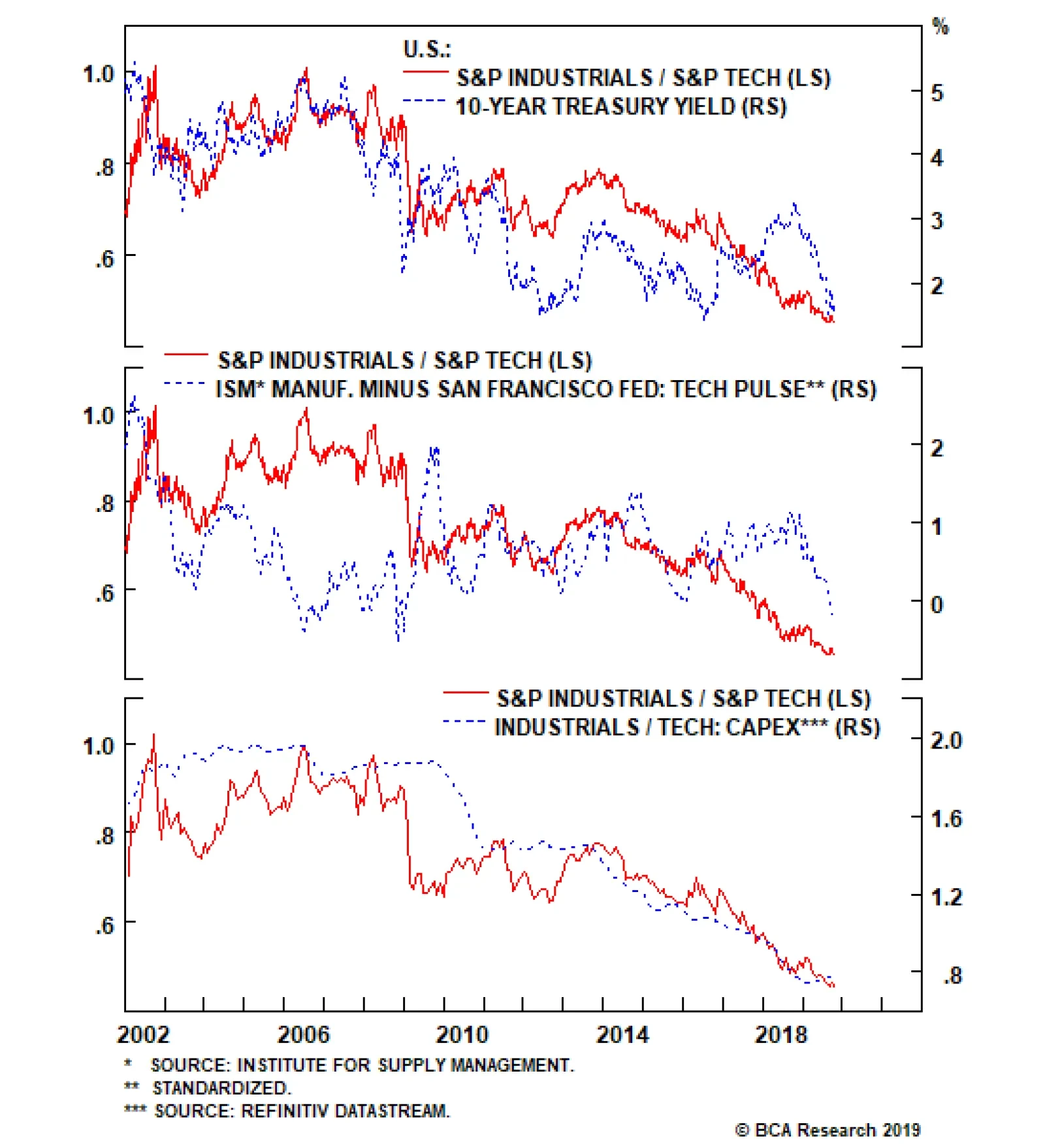
Trade War-Hedged Pair Trade (Part I) Trade War-Hedged Pair Trade (Part I) In this Monday’s Weekly Report we initiated a new long/short trade idea that will generate alpha regardless of the pair trade war outcome: long industrials/short tech. If the U.S. and China manage to iron out their differences and strike a deal, industrials should benefit from a greater catch-up phase because they have been depressed over the past two years, while tech stocks are near relative all-time highs. In contrast, a “no deal” scenario, should also re-concentrate investors’ minds and lead to relative selling in tech stocks versus their already beaten-down deep cyclical peers: industrials. Three key macro forces will be driving the rebound in the price ratio. First, were the deal to get struck, growth expectations will pick up pushing rates higher, which are a boon for industrials and a bane for high P/E tech stocks (top panel). Second, we expect the ISM manufacturing survey to outshine the San Francisco Fed’s Tech Pulse Index (middle panel). Finally, relative capital expenditure outlays should also veer in favor of industrials as previously mothballed infrastructure projects will come out of hibernation (bottom panel). On the other hand, should a “no-deal” scenario occur, we doubt that these three macro forces that we identified would sink further (please see the next Insight). ​​​​​​​

Highlights Portfolio Strategy The trade-weighted U.S. dollar’s appreciation along with the still souring manufacturing data are weighing on SPX profit growth, at a time when heightened geopolitical uncertainty and a looming reversal in financial conditions has the potential to wreak havoc on stock prices. Stay cautious on the prospects of the broad equity market on a cyclical 9-12 month time horizon. Firming operating metrics, the resilient U.S. dollar, compelling valuations and depressed technicals, all signal that there is an exploitable tactical trading opportunity in a long S&P industrials/short S&P tech pair trade, irrespective of the trade war outcome. A tentative tick up in EM and China data along with improving relative operating metrics signal that the time is ripe to initiate a long machinery/short semis pair trade. Recent Changes Initiate a long S&P Industrials/short S&P Tech pair trade on a tactical three-to-six month time horizon, today. Initiate a long S&P Machinery/short S&P Semiconductors pair trade on a tactical three-to-six month time horizon, today. Follow The Profit Trail Follow The Profit Trail Feature The S&P 500 oscillated violently again last week, as the barrage of declining economic data, heightened trade war-related volatility and political upheaval dominated the news flow. While the Fed remains the backstop of last resort, we doubt additional interest rate cuts, which are already aggressively priced in the bond market, will boost lending and entice CEOs to invest in capital expenditure projects. Investors have to stay patient and disciplined, let this economic slowdown play out and allow for the natural healing of the economy. As a reminder, the ISM manufacturing index has been decelerating for twelve months and only been below the boom bust line for two. If history is an accurate guide, an additional three-to-six months of manufacturing pain are in store before a definitive bottom is in place (bottom panel, Chart 1). Such a macro backdrop, still warrants caution on the prospects of the broad equity market. Chart 1Allow Time For Economic Healing Allow Time For Economic Healing Allow Time For Economic Healing Beginning in August, a number of BCA publications became a tad more cautious on risk assets. Following our October editorial view meeting last week, this cautiousness was cemented with a tactical downgrade of global equities to neutral from previously overweight in the BCA House View matrix. While this marks a clear shift toward this publication’s less sanguine view of the U.S. equity market adopted during the summer, BCA's cyclical 12-month House View remains overweight global equities. Worryingly, the majority of the indicators we track continue to emit distress signals and warn that the SPX has further downside (Chart 2), especially absent profit growth. Importantly, we first correctly posited last May that the back half of the year global growth reacceleration was in jeopardy and would go on hiatus courtesy of rising policy uncertainty.1 Such a backdrop would boost the U.S. dollar and simultaneously take a bite out of SPX EPS.2 Chart 2Soft Data Red Flag Soft Data Red Flag Soft Data Red Flag Last week we highlighted that the U.S. dollar is the most important indicator to monitor given its global deflationary/reflationary properties. Were the greenback to maintain its year-to-date gains, it will continue to dent SPX profitability via P&L translation loss effects and likely sustain the profit recession into early 2020 (trade-weighted U.S. dollar shown inverted, bottom panel, Chart 3). Chart 3Greenback Weighing On Profits Greenback Weighing On Profits Greenback Weighing On Profits U.S. Equity Strategy’s S&P 500 four-factor macro EPS growth model remains downbeat (middle panel, Chart 4). Were we to isolate the U.S. dollar as a single variable and re-run the regression it is clear that additional greenback appreciation will further weigh on SPX profit growth (bottom panel, Chart 4). Meanwhile, the easing in financial conditions and drubbing of the 10-year Treasury yield since the Christmas Eve lows is already reflected in the 23% jump in the forward PE multiple, which explains over 90% of the SPX’s rise since the Dec 24, 2018 trough (top & middle panels, Chart 5). In other words, for multiples to expand anew, financial conditions would have to further ease, which in our view is a tall order (bottom panel, Chart 5). Chart 4EPS Model Warrants Caution EPS Model Warrants Caution EPS Model Warrants Caution Chart 5Financial Conditions Are The Forward P/E Financial Conditions Are The Forward P/E Financial Conditions Are The Forward P/E This week we are initiating two related pair trades to exploit the mispricing of the trade war within the deep cyclical sector universe.  Thus, we would lean against the narrative that easy financial conditions are not fully reflected into stocks. In contrast, our worry is that junk spreads are on the verge of a breakout and such a backdrop would tighten financial conditions and aggravate an SPX drawdown (junk OAS shown inverted, Chart 6). Adding it all up, the trade-weighted U.S. dollar’s appreciation along with the still souring manufacturing data are weighing on SPX profit growth, at a time when heightened geopolitical uncertainty and a looming reversal in financial conditions has the potential to wreak havoc on stock prices. Stay cautious on the prospects of the broad equity market on a cyclical 9-12 month time horizon. This week we are initiating two related pair trades to exploit the mispricing of the trade war within the deep cyclical sector universe. Chart 6Watch Junk Spreads Watch Junk Spreads Watch Junk Spreads Initiate A Long Industrials/Short Tech Pair Trade… Ever since the Sino-American trade war started in March 2018, the market has punished industrials, but tech has escaped unscathed. While the global growth soft patch preceded the U.S./China trade spat, courtesy of the Fed’s tightening cycle and Chinese policymakers’ slamming on the brakes, the trade war has served as a catalyst to aggressively shed deep cyclical equities except for tech stocks (Chart 7). We think this misalignment presents a playable opportunity to generate alpha by going long industrials/short tech, irrespective of the trade war’s outcome. In other words, this market neutral trade will be in the black either because the trade spat gets resolved or because there will effectively be no “real” deal including intellectual property and the tech sector. If the two sides manage to iron out their differences and strike a deal, industrials stocks should benefit from a greater catch-up phase because they have been depressed over the past two years, while tech stocks are near relative all-time highs. In contrast, a “no deal” scenario, should also re-concentrate investors’ minds and lead to a relative selling in tech stocks versus their already beaten-down deep cyclical peers: industrials. Chart 7Bifurcated Deep Cyclicals Market Bifurcated Deep Cyclicals Market Bifurcated Deep Cyclicals Market Chart 8Lots Of Bad Trade War News Reflected In Prices Lots Of Bad Trade War News Reflected In Prices Lots Of Bad Trade War News Reflected In Prices Chart 8 shows the drubbing in relative share prices as three key macro drivers have felt the trade war’s wrath. In more detail, were a deal to get struck, growth expectations will reverse course and a bond market sell-off will almost immediately reflect such an improvement in the global macro backdrop. Rising interest rates on the back of a reflationary/inflationary impulse are a boon for industrials and a bane for high growth tech stocks (top panel, Chart 8). Similarly, the middle panel of Chart 8 highlights that the ISM manufacturing survey should climb above the boom/bust line and outshine the San Francisco Fed’s Tech Pulse Index (that comprises “coincident indicators of activity in the U.S. information technology sector”3) on news of a successful deal. Finally, relative capital expenditure outlays should also veer in favor of industrials as previously mothballed infrastructure projects will come out of hibernation (bottom panel, Chart 8). In contrast, tech capex has been resilient of late with analytics, security and cloud computing being the most defensive capex corner, leaving little room for additional relative capex gains. Taking the opposite side i.e. a “no deal”, we doubt the metrics we depict in Chart 8 would sink that much further. If anything we believe that there is an element of exhaustion and relative share prices would jump on news of a breakdown in trade talks as tech sector fire sales would trump the sell-off in already depressed industrials. Meanwhile, the U.S. dollar and relative share prices have been steeply diverging recently and this gap will likely narrow via a catch-up phase in the latter (top & middle panels, Chart 9). According to Factset’s latest data the S&P industrials sector garners 37% of its sales from abroad, whereas the S&P information technology sector’s foreign exposure stands at 57% of total revenues.4 Therefore, given this 20% delta, a rising greenback should be beneficial to the more domestically geared industrials stocks (bottom panel, Chart 9). On the operating front, industrials also have the upper hand. The relative wage bill is sinking like a stone (shown inverted, middle panel, Chart 10) at a time when relative selling price inflation is holding its own (top panel, Chart 10). The upshot is that a relative profit margin jump is in store in the coming months which should boost the relative share price ratio (bottom panel, Chart 10). 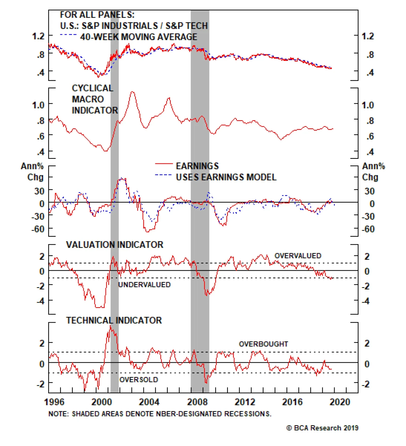Chart 9Unsustainable Divergence Unsustainable Divergence Unsustainable Divergence Chart 10Industrials Have The Upper Hand Industrials Have The Upper Hand Industrials Have The Upper Hand U.S. Equity Strategy’s proprietary relative Cyclical Macro Indicators and relative profit growth models capture all these drivers and both signal that an industrials versus tech earnings-led outperformance phase looms into year end (Chart 11). Chart 12 shows that the relative earnings breadth and relative net earnings revisions are both deep in negative territory. In terms of technicals, the relative percentage of groups trading with a positive 52-week rate of change has hit the lowest level in the past two decades (second panel, Chart 12) and our composite relative technical indicator is roughly one standard deviation below the historical mean (bottom panel, Chart 11). Chart 11Profit Models And...  Profit Models And...  Profit Models And...  Chart 12...Washed Out Breadth Say Buy Industrials At The Expense Of Tech ...Washed Out Breadth Say Buy Industrials At The Expense Of Tech ...Washed Out Breadth Say Buy Industrials At The Expense Of Tech Finally, relative valuations are also bombed out. Our relative valuation indicator has been in a six-year uninterrupted drop, falling from two standard deviations above the mean to one standard deviation below the mean (fourth panel, Chart 11). Such entrenched bearishness in relative value is unwarranted. Bottom Line:  Firming operating metrics, the resilient U.S. dollar, compelling valuations and depressed technicals, all signal that there is an exploitable tactical trading opportunity in a long S&P industrials/short S&P tech pair trade, irrespective of the trade war outcome. …And A Long Machinery/Short Semis Pair Trade A more speculative and higher octane vehicle to explore this trade war-related mispricing is via a long S&P machinery/short S&P semiconductors pair trade. Most of the drivers mentioned above also hold true in this subsector market-neutral trade. However, in this section we will drill deeper in the China/EM drivers. The Emerging Asia leading economic indicator (EALEI) has plummeted to levels last hit around the 1998 LTCM bailout (top panel, Chart 13). While more pain is likely in the coming months as global trade has ground to a halt, we doubt the carnage in the EALEI can continue indefinitely. In fact, a tentative trough in the Emerging Markets (EM) manufacturing PMI heralds a brighter outlook for relative share prices (bottom panel, Chart 13). Chart 13Same Trade War Theme, Different Vehicles To Play It Same Trade War Theme, Different Vehicles To Play It Same Trade War Theme, Different Vehicles To Play It Chart 14China...  China...  China...  Encouragingly, China’s fiscal and credit impulse also signals that a bottom in relative share prices is likely already in place. If this leading indicator proves accurate in the coming months, then relative share prices can spike 20% near the late-2018 highs (Chart 14).   Chinese money supply growth is showing some signs of life and capital committed to infrastructure spending is coming out of hibernation. Goldman Sachs’ China current activity indicator is on a similar upward trajectory, underscoring that the path of least resistance is higher for relative share prices (Chart 15). Chart 15...Holds The Key ...Holds The Key ...Holds The Key Chart 16Firming Final Demand... Firming Final Demand... Firming Final Demand... On the operating front, relative new orders and relative shipment growth have both ticked higher (top & middle panels, Chart 16). Importantly, our relative demand proxy suggests that the relative end-demand backdrop is also firming. Using Caterpillar’s global sales to dealers data compared with global chip sales reveals that a wide gap has formed between relative share prices and our relative demand gauge (bottom panel, Chart 16). If our thesis pans out in the upcoming three-to-six months then machinery will trounce semis. Finally, relative pricing power corroborates that machinery demand has the upper hand versus semiconductor final demand. The Commodity Research Bureau’s raw industrials index is climbing relative to Asian DRAM prices. The upshot is that the compellingly valued relative share price ratio will gain steam in the months ahead (Chart 17). In sum, a tentative up-tick in EM and China data along with improving relative operating metrics signal that the time is ripe to initiate a long machinery/short semis pair trade. Bottom Line: Initiate a long S&P machinery/short S&P semiconductors pair trade today. The ticker symbols for the stocks in the S&P machinery and S&P semis indexes are: BLBG – S5MACH – CAT, DE, ITW, IR, CMI, PCAR, PH, SWK, FTV, DOV, XYL, IEX, WAB, SNA, PNR, FLS, and BLBG – S5SECO – INTC, TXN, NVDA, AVGO, QCOM, MU, ADI, AMD, XLNX, QRVO, MCHP, MXIM, SWKS, respectively. Chart 17...Is A Boon To Relative Pricing Power ...Is A Boon To Relative Pricing Power ...Is A Boon To Relative Pricing Power Key Risk To Monitor One important risk to both of our newly recommended market-neutral trades is China. We recently touched base with our ex-Chief Geopolitical Strategist and currently Chief Strategist at the Clocktower Group, Marko Papic. He warned us that all bets would be off because: “I think we will look back at the recession of 2020 and it will be known as the “China recession”. Basically, China just decided to stop playing, pick up its toys, and go home”. If Marko’s wise words were to ring true, then such a Chinese policy shift will truly be a game changer with negative global economic growth implications. With regard to our pair trades, they would both be offside.   Anastasios Avgeriou, U.S. Equity Strategist anastasios@bcaresearch.com   Footnotes 1      Please see BCA U.S. Equity Strategy Weekly Report, “Consolidation” dated May 21, 2019, available at uses.bcaresearch.com. 2      Please see BCA U.S. Equity Strategy Weekly Report, “On Edge” dated May 13, 2019, available at uses.bcaresearch.com. 3      https://www.frbsf.org/economic-research/indicators-data/tech-pulse/ 4      https://www.factset.com/hubfs/Resources%20Section/Research%20Desk/Earnings%20Insight/EarningsInsight_100419A.pdf Current Recommendations Current Trades Size And Style Views Stay neutral cyclicals over defensives   (downgrade alert) Favor value over growth Favor large over small caps (Stop 10%)

Overweight Last week Costco reported its fiscal fourth-quarter earnings, which came in beating expectations. These results are good news for our S&P hypermarkets overweight call as Costco accounts for nearly 50% of the index. We first recommended investors increase their exposure to this plain vanilla consumer defensive industry just under 3 months ago, and this position is already up 8% relative to the SPX since inception. Macroeconomic data remains soft across the board heralding more gains for the S&P hypermarkets index (second panel). Meanwhile, industry specific data is encouraging, with Big Box retail sales slated to firm further (third & bottom panels). Specifically, hypermarkets’ pricing power is set to increase as the relative consumer confidence by income (defined as the ratio of Americans who make less than $35,000/annum to those who make above $35,000/annum) has climbed to fresh cyclical highs (bottom panel). Bottom Line: Consumer staples stocks in general and hypermarkets in particular continue to shine. Stay overweight the S&P hypermarkets index. The ticker symbols for the stocks in this index are: BLBG: S5HYPC - WMT, COST. Believe The Hype Believe The Hype    

Highlights The Chinese economy is still slowing, and there is not yet enough evidence from forward-looking economic data to suggest a turnaround is imminent. Deflation has returned to China’s industrial sector. Even though overall price deceleration has been relatively mild, it is further squeezing already deteriorating industrial profit growth. We do not expect deflation to spiral into a 2015/2016-style episode, which removes at least one risk to our growth outlook. At the same time, a mild deceleration in prices will not provide enough incentive for Chinese policymakers to hit the stimulus button.  The People’s Bank of China’s new interest rate-setting regime, the LPR, will not provide much in the way of stimulus over the next few months. But it has the potential to improve China’s monetary policy transmission mechanism over the coming year, increasing the odds that policymakers will succeed in stabilizing economic activity. Short-term downside risks to growth have not abated, and we remain tactically bearish on Chinese stocks. Cyclically, we continue to recommend an overweight stance, on the basis of an eventual reacceleration in economic activity. Feature Chart 1The Chinese Economy Is Still Slowing The Chinese Economy Is Still Slowing The Chinese Economy Is Still Slowing China’s economy is at a critical juncture: “Half-measured” stimulus so far has been able to keep the domestic economy in better shape than in the 2015-2016 down cycle, but overall economic activity has not bottomed (Chart 1). The Sino-America trade talk has resumed at the moment, but the two sides have yet to make any substantive progress towards a deal. In the meantime, the global economy has also reached a critical point where the degree of economic weakness has the potential to feed on itself, possibly triggering a recession.1  This underscores our tactically bearish stance towards Chinese stocks versus the global equity benchmark. Barring more forceful stimulus or resolution on the trade front, any external shock and/or internal policy missteps could easily tip the Chinese economy into a deeper growth slowdown. Hence, downside risks remain elevated for Chinese stocks over the next 3- to 6-months.    The “D” Word Returns, But Won’t Spur Aggressive Further Easing Chart 2Industrial Price Deflation Returns Industrial Price Deflation Returns Industrial Price Deflation Returns Economic data over the past two months have provided mixed signals. Readings from both China’s National Bureau of Statistics (NBS) PMI and from the Caixin PMI show an improvement in the manufacturing sector. However, industrial deflation has returned to China: Three years after the country declared victory against a prolonged industrial destocking cycle, producer price inflation (PPI) relapsed into negative territory in July and declined further in August (Chart 2).   While prices are typically lagging indicators and reflect lingering effects from past economic conditions, there is not enough evidence in forward-looking economic data right now to suggest a turnaround in the economy is imminent.2  A deflationary PPI is not a trivial source of concern for Chinese policymakers. Last time growth in China’s PPI turned negative, it took policymakers four and a half years and an annualized 28% of GDP worth of credit expansion to pull the industrial sector out of its deflationary cycle. Chart 3Deflation Threatens Recovery In Industrial Profit Growth Deflation Threatens Recovery In Industrial Profit Growth Deflation Threatens Recovery In Industrial Profit Growth For investors, deflation has pernicious effects on profits, and we have received several client inquiries concerning the topic since PPI growth turned negative. The historical relationship suggests profit growth for both the A-share and investable markets is highly linked to fluctuations in producer prices (Chart 3), and China’s industrial sector profit growth has already been rapidly deteriorating over the past 12 months. The good news is that we do not expect the current episode of PPI deflation to become as protracted as it did in 2012-2016, or as severe as in 2015-2016. Two reasons underpin our view: Since early-2018, monetary policy has been much easier than during past deflationary episodes. Monetary policy in the past year and half has been much more accommodative than in the three years leading to the deep industrial deflationary cycle in 2015, particularly on the exchange rate front. The RMB was soft-pegged to a rising U.S. dollar before it was decoupled by the PBoC in August 2015, and was appreciating against its trading partners throughout most of 2012-2015. Bank lending rates were also kept at historically high levels during this period (Chart 4). This time, even though money and credit growth has not returned to the same pace as in 2015-2016, current ultra-loose monetary conditions should spur enough credit growth to keep prices from deflating aggressively. Chart 4Monetary Conditions Easier Than Last Cycle Monetary Conditions Easier Than Last Cycle Monetary Conditions Easier Than Last Cycle Inventory levels are low, and capacity levels do not appear to be overly excessive. After years of industrial consolidation, China’s industrial capacity does not appear to be particularly excessive compared to the past cycle. This is distinctively different from the prolonged contraction in PPI between 2012 and 2016, when China’s industrial inventories were coming off a five-year-long destocking cycle, and capacity utilization fell markedly (Chart 5). This is not the case today. Moreover, even though final demand has been weak, production has retrenched even more, drawing down inventories to the point where the pace of inventory destocking may have reached a cyclical bottom (Chart 6). A re-stocking of industrial goods should boost producers’ pricing power. Chart 5Capacity Is Not Excessively Underutilized Capacity Is Not Excessively Underutilized Capacity Is Not Excessively Underutilized Chart 6Inventory Destocking May Be Bottoming Out Inventory Destocking May Be Bottoming Out Inventory Destocking May Be Bottoming Out But the bad news (for investors), is that contained, or mild producer price deflation will not be reason alone to spur aggressive further easing from policymakers. This means that the re-emergence of price deflation, even mild and short-lived, will weigh on earnings and investor sentiment. Bottom Line: This episode of producer price deflation is unlikely to become as pernicious as occurred in the past, but policymakers are thus unlikely to act aggressively to counter it. While this removes some of the downside risks for Chinese stocks, even mild deflation will weigh on earnings growth (and thus sentiment) which underscores our tactically bearish stance on Chinese stocks. Demystifying China’s New Loan Prime Rate: Not The Stimulus You Are Looking For On August 20th, the PBoC launched a new loan prime rate (LPR) system, a revamped reference regime for setting bank loan interest rates3 (Chart 7). In September, the new LPR rate for one-year bank loans was lowered by five basis points. Since then, the market has been fixated on predicting whether the PBoC will cut the Medium-Lending Facility (MLF) rate next, which would be perceived as a change in China’s monetary stance. Chart 7China's New LPR: A Shadow 'Tax Cut' China's New LPR: A Shadow "Tax Cut" China's New LPR: A Shadow "Tax Cut" PBoC will increase its control of the pricing of credit, while tight financial regulations will restrict the size and speed of credit growth. The new LPR reform, in our view, is designed to force state-owned (and better-capitalized) commercial banks to hand out a “tax cut” to struggling small- and medium-sized enterprises (SMEs) by lowering bank lending rates. At the same time, it allows the PBoC to take back control of the pricing of credit from commercial banks, “killing two birds with one stone.” There are three main market implications from this approach: The new LPR is likely to gradually narrow the gap between corporate bond yields (i.e. “market rates”) and bank lending rates; A cut in the MLF rate in the near term should be interpreted as a “reward” to commercial banks rather than a stimulus for the economy; Most importantly, the new LPR system does not mean rapid credit expansion is in the cards. Quite the opposite, in the near term, banks may tighten their lending. The wide spread between the 3-month interbank repo rate and average bank lending rate illustrates the reason why the PBoC has introduced the LPR.4 This gap is also evident when comparing the yield of AAA-rated corporate bonds and the average bank lending rate (Chart 8). These gaps exist because Chinese commercial banks have largely manipulated the 1-year bank lending rate set by the PBoC when lending to their “preferred customers,” usually state-owned enterprises and real estate developers, by offering significantly discounted loan rates. Banks then charge substantial “risk premiums” on loans to the private sector, mostly SMEs, to make up for the narrower profit margins on loans to SOEs (Chart 9). Chart 8An Impaired Monetary Policy Transmission Mechanism An Impaired Monetary Policy Transmission Mechanism An Impaired Monetary Policy Transmission Mechanism Chart 9Evidence Of Asymmetrical Lending Practices Evidence Of Asymmetrical Lending Practices Evidence Of Asymmetrical Lending Practices The new LPR system is designed to minimize this discrepancy, since the new LPRs are more market based and are quoted based on the price of loans banks charge their prime clients. By design, the new LPR system should force the average bank lending rate closer to the rate companies borrow in the bond market. This means bank lending rates will be guided lower, including lending rates for SMEs. However, the new system will be implemented in phases, and the PBoC is likely to gradually guide LPRs lower to allow banks to readjust their pricing models.  The LPR rate is essentially the MLF rate plus bank profit margins (the added basis points above the MLF rate). The market will guide the top line lending rate, while the PBoC will have control over the floor rate (MLF) through open market operations. The fact that the PBoC is keeping the MLF rate unchanged while allowing the LPR to drop (albeit slightly) sends an explicit message: The PBoC is forcing banks to lower lending rates first before boosting their now-narrowed profit margins by lowering the MLF rate. In contrast to expectations of market participants that the LPR system will ease credit conditions, banks may actually tighten their lending in the coming months. While the PBoC will increase its control of the pricing of bank loans by the rate reform plan, the strengthening in financial regulations that has occurred over the past year will restrict the size and speed of credit growth. This combination has created more room for monetary easing without unleashing “animal spirits.” Borrowing costs to risky institutions have been higher since the Baoshang Bank takeover and are likely to remain elevated even if interest rates are lower (Chart 10). More importantly, mortgage and real estate developer loans together account for nearly 30% of total bank credit. Unless policymakers ease the brakes on lending restrictions to the property sector, bank lending growth is unlikely to pick up meaningfully (Chart 11). In fact, the PBoC has explicitly excluded mortgage and property-related lending from benefitting from the LPR rate cut.5 Barring a significant worsening in economic data, we do not expect the PBoC to lower mortgage lending and real estate-related loan rates in the coming months. Chart 10Tightened Financial Regulations Will Keep Cost Of Risky Lending High Tightened Financial Regulations Will Keep Cost Of Risky Lending High Tightened Financial Regulations Will Keep Cost Of Risky Lending High Chart 11Mortgage Rate Unlikely To Return To Its 2016 Low Mortgage Rate Unlikely To Return To Its 2016 Low Mortgage Rate Unlikely To Return To Its 2016 Low Finally, in the next two- to three-quarter mandatory implementation period, banks will be readjusting their pricing and credit risk-assessing models. During the transition, we expect more cautious sentiment among both lenders and borrowers. Hence, in the short term, bank loan growth may actually moderate. Bottom Line: The new LPR system may lower China’s banking sector profits in the short term. But in the next 6- to 12-months, we expect the PBoC to compensate commercial banks by keeping ample liquidity in the interbank system and by eventually lowering the MLF rate. The new LPR system may slow bank credit growth in the next few months, but after its full implementation (by the second quarter of 2020), it will have the potential to make PBoC’s policy more effective. Investment Conclusions We expect two phases of Chinese equity relative performance over the coming year: one phase of flat-to-potentially seriously down performance to last from now until sometime in the first quarter of 2020 when the economy bottoms, and then a phase of outperformance. Our expectation that the economy will bottom in Q1 2020 rests on the existing reflationary response by Chinese policymakers and an improved monetary transmission mechanism. Chart 12We Expect The Chinese Economy To Bottom In Q1 2020 We Expect The Chinese Economy To Bottom In Q1 2020 We Expect The Chinese Economy To Bottom In Q1 2020 Our expectation that the economy will bottom in the first quarter of 2020 continues to rest on the existing reflationary response by Chinese policymakers (Chart 12), and the fact that China’s new LPR system has the potential to improve what is currently a seriously impaired monetary transmission mechanism beyond the next two or three quarters. But the existing response of policymakers has been considerably more measured when compared to past economic cycles, meaning that equity investors are unlikely to be as forward-looking as they otherwise might be. Weak producer price deflation will weigh on investor sentiment, and it is unlikely to be weak enough to spur aggressive further easing. The potential for further escalation of the U.S.-China trade war also compellingly argues against an overweight stance in the near-term, even if we expect economic growth to subsequently improve. Consequently, we remain tactically bearish and cyclically bullish towards Chinese stocks: medium-term investors who are already positioned in favor of China-related assets should stay long, whereas investors who have not yet moved to an overweight stance should wait for a better buying opportunity to emerge over the coming few months.   Jing Sima China Strategist JingS@bcaresearch.com     Footnotes 1      Please see Global Investment Strategy Outlook “Fourth Quarter 2019 Strategy Outlook: A “Show Me” Market”, dated October 4, 2019, available at gis.bcaresearch.com 2      Please see China Investment Strategy Weekly Report “China Macro And Market Review”, dated October 2, 2019, available at cis.bcaresearch.com 3      Announcement of the People’s Bank of China on Improving Loan Prime Rate (LPR) Formation Mechanism, August 19, 2019, available at http://www.pbc.gov.cn/en/3688110/3688172/3877490/index.html 4      PBC Official Answers Press Questions on Improving Loan Prime Rate (LPR) Formation Mechanism, August 20, 2019, available at http://www.pbc.gov.cn/en/3688110/3688172/3877865/index.html 5      Announcement of the People’s Bank of China No.16, August 27, 2019, available at http://www.pbc.gov.cn/en/3688110/3688172/3881177/index.html Cyclical Investment Stance Equity Sector Recommendations

Highlights Q3/2019 Performance Breakdown: Our recommended model bond portfolio underperformed the custom benchmark by -30bps during the third quarter of the year. Winners & Losers: The biggest underperformance came from underweight positions in U.S. Treasuries (-28bps) and Italian government bonds (-18bps) as yields plunged, dwarfing gains from overweights in corporate bonds in the U.S. (+11bps) and euro area (+4bps). Scenario Analysis For The Next Six Months: We are maintaining our current positioning, staying below-benchmark on duration while overweighting U.S. and euro area corporates vs. government debt. In our base case scenario, global growth will begin to stabilize but the Fed will deliver one more “insurance” rate cut by year-end, leading to corporate bond outperformance. Feature Global bond markets have enjoyed a powerful bull run throughout 2019, as yields have plummeted alongside weakening global growth and growing political uncertainty. Those two forces came to a head in the third quarter of the year, with U.S.-China trade tensions ratcheting up another notch after the imposition of higher U.S. tariffs in early August and global manufacturing PMI data moving into contraction territory – especially in the U.S. The result was a significant fall in government bond yields as markets discounted both lower inflation expectations and more aggressive monetary easing from global central banks, led by the Fed and ECB. The benchmark 10-year U.S. Treasury yield and 10-year German Bund yield plunged -40bps and -25bps, respectively, during the July-September period. Yet at the same time, global credit markets remained surprisingly stable, as the option-adjusted spread on the Bloomberg Barclays Global Corporates index was unchanged over the same three months. In this report, we review the performance of the BCA Global Fixed Income Strategy (GFIS) model bond portfolio during the eventful third quarter of 2019. We also present our updated scenario analysis, and total return projections, for the portfolio over the next six months. As a reminder to existing readers (and to new clients), the model portfolio is a part of our service that complements the usual macro analysis of global fixed income markets. The portfolio is how we communicate our opinion on the relative attractiveness between government bond and spread product sectors. This is done by applying actual percentage weightings to each of our recommendations within a fully invested hypothetical bond portfolio. Q3/2019 Model Portfolio Performance Breakdown: Good News On Credit Trumped By Bad News On Duration Chart of the WeekDuration Losses Dwarf Credit Gains In Q3/19 Duration Losses Dwarf Credit Gains In Q3/19 Duration Losses Dwarf Credit Gains In Q3/19 The total return for the GFIS model portfolio (hedged into U.S. dollars) in the third quarter was 2.0%, lagging the custom benchmark index by -30 bps (Chart of the Week).1 This brings the cumulative year-to-date total return of the portfolio to +7.8%, which has underperformed the benchmark by a disappointing –67bps. The Q3 drag on relative returns came entirely from the government bond side of the portfolio; specifically, the underweight allocation to U.S. Treasuries and Italian government bonds (Table 1). Those allocations reflected our views on overall portfolio duration (below benchmark) and a relative value consideration within European spread product (preferring corporates to Italy). Both those recommendations went against us as global bond yields dropped during Q3, with Italian yields collapsing (the benchmark 10-year yield was down –126bps) as investors chased any positive yield denominated in euros after the ECB signaled a new round of policy easing. The total return for the GFIS model portfolio (hedged into U.S. dollars) in the third quarter was 2.0%, lagging the custom benchmark index by -30 bps  Table 1GFIS Model Bond Portfolio Q3/2019 Overall Return Attribution Q3/2019 GFIS Model Bond Portfolio Performance Review: More Duration/Credit Divergence Q3/2019 GFIS Model Bond Portfolio Performance Review: More Duration/Credit Divergence Providing some partial offset to the U.S. and Italy allocations were gains from overweight positions in government bonds in the U.K., Australia and Japan. More importantly, our overweights in corporate debt in the U.S. and euro area made a strong positive contribution to the performance of the portfolio. The bar charts showing the total and relative returns for each individual government bond market and spread product sector are presented in Charts 2 and 3. The most significant movers were: Chart 2GFIS Model Bond Portfolio Q3/2019 Government Bond Performance Attribution Q3/2019 GFIS Model Bond Portfolio Performance Review: More Duration/Credit Divergence Q3/2019 GFIS Model Bond Portfolio Performance Review: More Duration/Credit Divergence Chart 3GFIS Model Bond Portfolio Q3/2019 Spread Product Performance Attribution By Sector Q3/2019 GFIS Model Bond Portfolio Performance Review: More Duration/Credit Divergence Q3/2019 GFIS Model Bond Portfolio Performance Review: More Duration/Credit Divergence Biggest outperformers Overweight U.S. high-yield Ba-rated (+4bps) Overweight U.S. high-yield B-rated (+3bps) Overweight U.S. investment grade industrials (+3bps) Overweight Japanese government bonds with maturity of 5-7 years (+2bps) Overweight euro area corporates, both investment grade (+2bps) and high-yield (+2bps) Biggest underperformers Underweight U.S. government bonds with maturity beyond 10+ years (-15bps) Underweight Italy government bonds with maturity beyond 10+ years (-10bps) Underweight U.S. government bonds with maturity of 7-10 years (-5bps) Underweight Japanese government bonds with maturity beyond 10+ years (-4bps) Underweight U.S. government bonds with maturity of 3-5 years (-4bps) Chart 4 presents the ranked benchmark index returns of the individual countries and spread product sectors in the GFIS model bond portfolio for Q3/2019. The returns are hedged into U.S. dollars (we do not take active currency risk in this portfolio) and are adjusted to reflect duration differences between each country/sector and the overall custom benchmark index for the model portfolio. We have also color-coded the bars in each chart to reflect our recommended investment stance for each market during Q3/2019 (red for underweight, blue for overweight, gray for neutral).2 Ideally, we would look to see more blue bars on the left side of the chart where market returns are highest, and more red bars on the right side of the chart were returns are lowest. Chart 4Ranking The Winners & Losers From The Model Bond Portfolio In Q3/2019 Q3/2019 GFIS Model Bond Portfolio Performance Review: More Duration/Credit Divergence Q3/2019 GFIS Model Bond Portfolio Performance Review: More Duration/Credit Divergence One thing that stands out from Chart 4 is that every fixed income sector generated a positive return, except for EM USD-denominated corporates. This is a fascinating outcome given the sharp falls in risk-free government bond yields which typically would correlate to a selloff in risk assets and widening of credit spreads. The soothing balm of looser global monetary policy seems to have offset the impact of elevated uncertainty on trade and future economic growth, allowing both bond yields and credit spreads to stay low. The soothing balm of looser global monetary policy seems to have offset the impact of elevated uncertainty on trade and future economic growth, allowing both bond yields and credit spreads to stay low.  We maintained an overweight stance on global spread product throughout Q3, as we felt that the monetary policy effect would continue to overwhelm uncertainty. We did, however, make some tactical adjustments to our duration stance after the U.S. raised tariffs on Chinese imports, upgrading to neutral on August 6th.3 We had felt that higher tariffs were a sign that a potential end to the U.S.-China trade conflict was now even less likely, which raised the odds of a potential risk-off financial market event that would temporarily push bond yields lower. We shifted back to a below-benchmark duration stance on September 17th, given signs of de-escalation in the trade dispute and, more importantly, some improvement evident in global leading economic indicators.4 Bottom Line: Our recommended model bond portfolio underperformed the custom benchmark index during the third quarter of the year, with the drag on performance from an underweight stance on U.S. Treasuries and Italian BTPs overwhelming the gains from corporate credit overweights in the U.S. and euro area. Future Drivers Of Portfolio Returns Looking ahead, the performance of the model bond portfolio will continue to be driven by two main factors: our below-benchmark duration bias and our overweight stance on global corporate debt versus government bonds. Chart 5Overall Portfolio Allocation: Overweight Credit Q3/2019 GFIS Model Bond Portfolio Performance Review: More Duration/Credit Divergence Q3/2019 GFIS Model Bond Portfolio Performance Review: More Duration/Credit Divergence In terms of the specific high-level weightings in the model portfolio, we currently have a moderate overweight, equal to eight percentage points, on spread product versus government debt (Chart 5). This reflects a more constructive view on future global growth. Early leading economic indicators are starting to bottom out and global central bankers are maintaining a dovish policy bias despite low unemployment rates – both factors that will continue to benefit growth-sensitive assets like corporate debt. Early leading economic indicators are starting to bottom out and global central bankers are maintaining a dovish policy bias despite low unemployment rates – both factors that will continue to benefit growth-sensitive assets like corporate debt. We are maintaining our below-benchmark duration tilt at 0.6 years short of the custom benchmark (Chart 6). We recognize, however, that the underperformance from duration in the model portfolio will not begin to be clawed back until there are signs of a bottoming in widely-followed cyclical economic indicators like the U.S. ISM index and the German ZEW. We think that will happen given the uptick in our global leading economic indicator (LEI), but that may take a few more months to develop based on the usual lead time from the LEI to the survey data like the ISM. The hook up in the global LEI does still gives us more confidence that the big decline in global bond yields seen this year is over, especially if a potential truce in the U.S.-China trade war is soon reached, as our political strategists believe to be increasingly likely. Chart 6Overall Portfolio Duration: Moderately Below Benchmark Overall Portfolio Duration: Moderately Below Benchmark Overall Portfolio Duration: Moderately Below Benchmark Turning to country allocation, we are sticking with overweights in countries where central banks are likely to be more dovish than the Fed over the next 6-12 months (Germany, France, the U.K., Japan, and Australia). We are staying underweight the U.S. where inflation expectations appear too low and Fed rate cut expectations look too extreme. The Italy underweight has become a trickier call. We have long viewed Italian debt as a growth-sensitive credit instrument rather than the yield-driven rates vehicle it became in Q3 as markets priced in fresh monetary easing measures from the ECB (including restarting government purchases). We will revisit our Italy views in an upcoming report but, until then, we will continue to view Italian BTPs within the context of our European spread product allocation. Thus, we are maintaining an overweight on euro area corporate debt (by 1% each in investment grade and high-yield) while having an equal-sized underweight (-2%) in Italian government bonds. Our combined positioning generates a portfolio that has “positive carry”, with a yield of 3.1% (hedged into U.S. dollars) that is +25bps over that of the custom benchmark index (Chart 7). That same portfolio, however, generates an estimated tracking error (excess volatility of the portfolio versus its benchmark) of 55bps - well below our self-imposed 100bps ceiling and still within the 40-60bps range we have targeted since the start of 2019 (Chart 8). Chart 7Portfolio Yield: Positive Carry From Credit Portfolio Yield: Positive Carry From Credit Portfolio Yield: Positive Carry From Credit Chart 8Portfolio Risk Budget Usage: Cautious Portfolio Risk Budget Usage: Cautious Portfolio Risk Budget Usage: Cautious Scenario Analysis & Return Forecasts In April 2018, we introduced a framework for estimating total returns for all government bond markets and spread product sectors, based on common risk factors.5 For credit, returns are estimated as a function of changes in the U.S. dollar, the Fed funds rate, oil prices and market volatility as proxied by the VIX index (Table 2A). For government bonds, non-U.S. yield changes are estimated using historical betas to changes in U.S. Treasury yields (Table 2B). Table 2AFactor Regressions Used To Estimate Spread Product Yield Changes Q3/2019 GFIS Model Bond Portfolio Performance Review: More Duration/Credit Divergence Q3/2019 GFIS Model Bond Portfolio Performance Review: More Duration/Credit Divergence Table 2BEstimated Government Bond Yield Betas To U.S. Treasuries Q3/2019 GFIS Model Bond Portfolio Performance Review: More Duration/Credit Divergence Q3/2019 GFIS Model Bond Portfolio Performance Review: More Duration/Credit Divergence This framework allows us to conduct scenario analysis of projected returns for each asset class in the model bond portfolio by making assumptions on those individual risk factors. In Tables 3A & 3B, we present our three main scenarios for the next six months, defined by changes in the risk factors, and the expected performance of the model bond portfolio in each case. The scenarios, described below, all revolve around our expectation that the most important drivers of future market returns will continue to be the momentum of global growth and the path of U.S. monetary policy. The scenario inputs for the four main risk factors (the fed funds rate, the price of oil, the U.S. dollar and the VIX index) are shown visually in Chart 9. Table 3AScenario Analysis For The GFIS Model Bond Portfolio For The Next Six Months Q3/2019 GFIS Model Bond Portfolio Performance Review: More Duration/Credit Divergence Q3/2019 GFIS Model Bond Portfolio Performance Review: More Duration/Credit Divergence Table 3BU.S. Treasury Yield Assumptions For The 6-Month Forward Scenario Analysis Q3/2019 GFIS Model Bond Portfolio Performance Review: More Duration/Credit Divergence Q3/2019 GFIS Model Bond Portfolio Performance Review: More Duration/Credit Divergence Chart 9Risk Factor Assumptions For The Scenario Analysis Risk Factor Assumptions For The Scenario Analysis Risk Factor Assumptions For The Scenario Analysis Base Case (Global Growth Bottoms): The Fed delivers one more -25bp rate cut by the end of 2019, the U.S. dollar weakens by -3%, oil prices rise by +10%, the VIX hovers around 15, and there is a bear-steepening of the UST curve. This is a scenario where the U.S. economy ends up avoiding recession and grows at roughly a trend-like pace. The Fed, however, still delivers one more “insurance” rate cut to mitigate the risk of low inflation expectations becoming more entrenched. Global growth is expected to bottom out as heralded by the global leading indicators. A truce (but not a full deal) is expected on the U.S.-China trade front, helping to moderately soften the U.S. dollar through reduced risk aversion. The model bond portfolio is expected to beat the benchmark index by +91bps in this case. Global Growth Strongly Rebounds: The Fed stays on hold, the U.S. dollar weakens by -5%, oil prices rise by +20%, the VIX declines to 12, there is a modest bear-steepening of the UST curve. In this tail-risk scenario, global growth starts to reaccelerate in lagged response to the global monetary easing seen this year, combined with some fiscal stimulus in major countries (China, the U.S., perhaps even Germany). The U.S. dollar weakens as global capital flows shift to markets which are more sensitive to global growth. The model bond portfolio is expected to beat the benchmark index by +106bps in this case. U.S. Downturn Intensifies: The Fed cuts rates by -75bps, the U.S. dollar is flat, oil prices fall by -15%, the VIX rises to 30; there is a bull-steepening of the UST curve. Under this tail-risk scenario, the current slowing of U.S. growth momentum gains speed, pushing the economy towards recession. The Fed cuts rates aggressively in response, helping weaken the U.S. dollar, but not before global risk assets sell off sharply to discount a worldwide recession. The model portfolio will underperform the benchmark by -38bps in this scenario. In terms of our conviction level among the main drivers of the model portfolio returns – duration allocation (across yield curves and countries) and asset allocation (credit versus government bonds) – we are most confident that credit returns will exceed those of sovereign debt over the next six months. In terms of our conviction level among the main drivers of the model portfolio returns – duration allocation (across yield curves and countries) and asset allocation (credit versus government bonds) – we are most confident that credit returns will exceed those of sovereign debt over the next six months. The underweight duration position, however, will also eventually begin to pay off if the message from the budding improvement in global leading economic indicators turns out to be correct. A collapse of the U.S.-China trade negotiations is the biggest threat to our base case, which would make the “U.S. Downturn Intensifies” scenario a more likely outcome. Bottom Line: We are maintaining our current positioning, staying below-benchmark on duration while overweighting U.S. and euro area corporates governments. In our base case scenario, global growth will begin to stabilize but the Fed will deliver one more “insurance” rate cut by year-end, leading to spread product outperformance.   Robert Robis, CFA, Chief Fixed Income Strategist rrobis@bcaresearch.com Ray Park, CFA, Research Analyst ray@bcaresearch.com Footnotes 1 The GFIS model bond portfolio custom benchmark index is the Bloomberg Barclays Global Aggregate Index, but with allocations to global high-yield corporate debt replacing very high quality spread product (i.e. AA-rated). We believe this to be more indicative of the typical internal benchmark used by global multi-sector fixed income managers. 2 Note that sectors where we made changes to our recommended weightings during Q3/2019 will have multiple colors in the respective bars in Chart 4. 3 Please see BCA Global Fixed Income Strategy Weekly Report, “Trade War Worries: Once More, With Feeling”, dated August 6, 2019, available at gfis.bcaresearch.com. 4 Please see BCA Global Fixed Income Strategy Weekly Report, “The World Is Not Ending: Return To Below-Benchmark Portfolio Duration”, dated September 17, 2019, available at gfis.bcaresearch.com. 5 Please see BCA Global Fixed Income Strategy Weekly Report, “GFIS Model Bond Portfolio Q1/2018 Performance Review: A Rough Start”, dated April 10th 2018, available at gfis.bcareseach.com. Recommendations The GFIS Recommended Portfolio Vs. The Custom Benchmark Index Q3/2019 GFIS Model Bond Portfolio Performance Review: More Duration/Credit Divergence Q3/2019 GFIS Model Bond Portfolio Performance Review: More Duration/Credit Divergence Duration Regional Allocation Spread Product Tactical Trades Yields & Returns Global Bond Yields Historical Returns

Highlights Chart 1Contagion? Contagion? Contagion? Until last week, global growth weakness had been wholly confined to the manufacturing sector. But the drop to 52.6 in September’s Non-Manufacturing PMI (from 56.4 in August) raises the specter of contagion from manufacturing into the broader U.S. economy. A further drop would be consistent with an economy headed toward recession, and run contrary to the 2015/16 roadmap that has been our base case (Chart 1). We think it is still premature to abandon the 2015/16 episode as an appropriate comparable for the current period. For one thing, the hard economic data paint a rosier picture than the PMI surveys. Industrial production and core durable goods new orders are up 2.5% and 2.3% (annualized), respectively, during the past 3 months. These data have helped drive the economic surprise index above zero, an event that usually coincides with rising yields (bottom panel). The divergence between soft and hard data makes it clear that trade uncertainties are so far having a greater impact on business sentiment than on actual production, but history tells us that these divergences don’t last long. Some positive news on the trade front will be required during the next few months to raise business sentiment and push bond yields higher. Stay tuned. Feature Investment Grade: Overweight Chart 2Investment Grade Market Overview Investment Grade Market Overview Investment Grade Market Overview Investment grade corporate bonds outperformed the duration-equivalent Treasury index by 42 basis points in September, before giving back 37 bps in the first week of October. We consider three main factors in our credit cycle analysis: (i) corporate balance sheet health, (ii) monetary conditions, and (iii) valuation. At present, the chief conundrum for investors is that while corporate balance sheet health is weak, the monetary environment is extraordinarily accommodative.1 On balance sheets, our top-down measure of gross leverage is elevated and rising (Chart 2). In contrast, interest coverage ratios remain solid, propped up by the Fed’s accommodative stance. With inflation expectations still very low, the Fed can maintain its “easy money” policy for some time yet. This will ensure that interest coverage stays solid and that bank lending standards continue to ease (bottom panel). This is an environment where corporate bond spreads should tighten. How low can spreads go? Our assessment of reasonable spread targets for the current environment suggests that Aaa, Aa and A-rated spreads are already fully valued, while Baa-rated spreads are 13 bps cheap (panels 2 & 3).2 We recommend focusing investment grade corporate bond exposure on the Baa credit tier, and subbing some Agency MBS into your portfolio in place of corporate bonds rated A or higher. Table 3ACorporate Sector Relative Valuation And Recommended Allocation* Crunch Time Crunch Time Table 3BCorporate Sector Risk Vs. Reward* Crunch Time Crunch Time High-Yield: Overweight Chart 3High-Yield Market Overview High-Yield Market Overview High-Yield Market Overview High-Yield outperformed the duration-equivalent Treasury index by 66 basis points in September, before giving back 117 bps in the first week of October. The junk index’s option-adjusted spread (OAS) has been fairly stable for most of the year, but the sector has become increasingly attractive from a risk/reward perspective.3 This is because the index’s negatively convex nature has caused its average duration to fall alongside declining Treasury yields. Chart 3 shows that while the index OAS has been rangebound, the 12-month breakeven spread has widened considerably.4 In other words, while junk expected returns have been stable, those expected returns now come with considerably less risk. As a result, the junk index OAS looks increasingly attractive relative to our spread target.5 Specifically, we now view the junk index OAS as 171 bps cheap (panel 3). Falling index duration also explains the divergence between quality spreads and the index OAS. Many have observed that the spread differential between Caa and Ba-rated junk bonds has widened in recent months, while the overall index OAS has been stable (panel 4). However, the divergence evaporates when we look at 12-month breakeven spreads instead of OAS (bottom panel). MBS: Neutral Chart 4MBS Market Overview MBS Market Overview MBS Market Overview Mortgage-Backed Securities outperformed the duration-equivalent Treasury index by 24 basis points in September, before giving back 25 bps in the first week of October. MBS have underperformed Treasuries by 31 bps, year-to-date. The conventional 30-year zero volatility spread held flat at 82 bps in September, as a 3 bps increase in expected prepayment losses (option cost) was offset by a 3 bps tightening in the option-adjusted spread (OAS). In last week’s report, we recommended favoring Agency MBS over Aaa, Aa and A-rated corporate bonds.6 We have three main reasons for this recommendation. First, expected compensation is competitive. The conventional 30-year MBS OAS is now 57 bps. This is above the pre-crisis average (Chart 4), and only 4 bps below the spread offered by a Aa-rated corporate bond. Aaa, Aa and A-rated corporate bond spreads also all look expensive relative to our targets. Second, risk-adjusted compensation heavily favors MBS. The 12-month breakeven spread for a conventional 30-year MBS is 21 bps. This compares to 6 bps, 8 bps and 12 bps for Aaa, Aa and A-rated corporates, respectively. Finally, the macro environment for MBS remains supportive. Mortgage lending standards have barely eased since the financial crisis (bottom panel), and most people have already had at least one opportunity to refinance their mortgage. This burnout will keep refi activity low, and MBS spreads tight (panel 2), going forward. Government-Related: Underweight Chart 5Government-Related Market Overview Government-Related Market Overview Government-Related Market Overview The Government-Related index outperformed the duration-equivalent Treasury index by 10 basis points in September, bringing year-to-date excess returns up to +163 bps. September returns were concentrated in the Foreign Agency sub-sector. These securities outperformed the Treasury benchmark by 55 bps on the month, bringing year-to-date excess returns up to +197 bps. Sovereign bonds underperformed duration-equivalent Treasuries by 6 bps in September, dragging year-to-date excess returns down to +436 bps. Local Authority and Domestic Agency debt underperformed by 1 bp and 2 bps on the month, respectively. Meanwhile, Supranationals bested the Treasury benchmark by a single basis point. Sovereign debt remains very expensive relative to equivalently-rated U.S. corporate credit (Chart 5). While the sector would benefit if the Fed’s dovish pivot eventually results in a weaker dollar, U.S. corporate bonds would also perform well in such an environment. Given the much more attractive starting point for U.S. corporate bond spreads, we find it difficult to recommend sovereign debt as an alternative. While sovereign debt in general looks expensive. USD-denominated Mexican sovereign bonds continue to look attractive relative to U.S. corporates (bottom panel). Investors should favor Mexican sovereigns within an otherwise underweight allocation to the sector as a whole. Municipal Bonds: Overweight Chart 6Municipal Market Overview Municipal Market Overview Municipal Market Overview Municipal bonds underperformed the duration-equivalent Treasury index by 10 basis points in September, dragging year-to-date excess returns down to -57 bps (before adjusting for the tax advantage). We recommended upgrading municipal bonds from neutral to overweight in last week’s report.7  We based the decision on the increasing attractiveness of yield ratios, despite an underlying credit environment that remains supportive for munis. Municipal bond yields failed to keep pace with falling Treasury yields in recent months, and now look quite attractive as a result (Chart 6). The average Aaa-rated Municipal / Treasury (M/T) yield ratio rose 4% in September and is now back above 90%. This is well above the 81% average that prevailed in the late stages of the previous cycle, between mid-2006 and mid-2007. In fact, Aaa M/T yield ratios for every maturity are now above average pre-crisis levels. Though yield ratios still look best at the long-end of the Aaa curve (panel 2), we now recommend owning munis in place of Treasuries across the entire maturity spectrum. Fundamentally, state & local government balance sheets remain solid. We showed in last week’s report that our Municipal Health Monitor is in “improving health” territory, and noted that state & local government interest coverage is positive (bottom panel). Both of those trends are consistent with muni ratings upgrades continuing to outnumber downgrades going forward. Treasury Curve: Maintain A Barbell Curve Positioning Chart 7Treasury Yield Curve Overview Treasury Yield Curve Overview Treasury Yield Curve Overview The Treasury curve bear-steepened in September, and then bull-steepened sharply last week. All in all, the 2/10 Treasury slope is +12 bps, 12 bps steeper than it was at the end of August. The 5/30 slope is +67 bps, 10 bps steeper than at the end of August. Our fair value models (see Appendix B) continue to show that bullets are expensive relative to barbells across the entire Treasury curve. In particular, 5-year and 7-year maturities look very expensive compared to the short and long ends of the curve. Notice that the 2/5/10 butterfly spread, the spread between the 5-year bullet and a duration-matched 2/10 barbell, remains negative despite the recent 2/10 steepening (Chart 7). We have shown in prior research that the 5-year and 7-year maturities are the most highly correlated with our 12-month Fed Funds Discounter. Our discounter is currently at -74 bps, meaning that the market is priced for nearly three more Fed rate cuts during the next 12 months (top panel). We expect fewer cuts than that, and as such, think the Discounter is more likely to rise. 5-year and 7-year maturities would underperform the rest of the curve in that scenario. We also continue to hold our short position in the February 2020 fed funds futures contract. That contract is currently priced for 2 more rate cuts during the next 3 FOMC meetings. That outcome is possible, but our base case economic outlook is more consistent with 1 further cut, likely occurring this month. TIPS: Overweight Chart 8Inflation Compensation Inflation Compensation Inflation Compensation TIPS underperformed the duration-equivalent nominal Treasury index by 38 basis points in September, dragging year-to-date excess returns down to -142 bps. The 10-year TIPS breakeven inflation rate fell 3 bps in September, and then another 2 bps last week. It currently sits at 1.51%, well below levels consistent with the Fed’s target. The divergence between the actual inflation data and inflation expectations is becoming increasingly stark. Trimmed mean PCE inflation has been fluctuating around the Fed’s target for most of the year (Chart 8). However, long-maturity TIPS breakeven inflation rates remain stubbornly low, nowhere near the 2.3% - 2.5% range that is consistent with the Fed’s target. As we have pointed out in prior research, it can take time for expectations to adapt to a changing macro environment.8 That being said, the 10-year TIPS breakeven inflation rate is currently 43 bps too low according to our Adaptive Expectations Model, a model whose primary input is 10-year trailing core inflation (panel 4). It is highly likely that the Fed will have to tolerate some overshoot of its 2% inflation target in order to re-anchor inflation expectations near desired levels. We anticipate that the committee will do so, and we maintain our view that long-dated TIPS breakevens will move above 2.3% before the end of the cycle. ABS: Underweight Chart 9ABS Market Overview ABS Market Overview ABS Market Overview Asset-Backed Securities underperformed the duration-equivalent Treasury index by 2 basis points in September, dragging year-to-date excess returns down to +72 bps. The index option-adjusted spread for Aaa-rated ABS widened 2 bps on the month. It currently sits at 36 bps, very close to its minimum pre-crisis level (Chart 9). ABS also appear unattractive on a risk/reward basis, as both Aaa-rated auto loans and credit cards have moved into the “Avoid” quadrant of our Excess Return Bond Map (Appendix C). The Map uses each bond sector’s spread, duration and volatility to calculate the likelihood of earning or losing 100 bps of excess return versus Treasuries on a 12-month horizon. At present, the Map shows that ABS offer poor expected return for their level of risk. In addition to poor valuation, the ABS sector’s credit fundamentals are shifting in a negative direction. Household interest payments continue to trend up, suggesting a higher delinquency rate in the future (panel 3). Meanwhile, senior loan officers continue to tighten lending standards for both credit cards and auto loans. Tighter lending standards usually coincide with rising delinquencies (bottom panel). All in all, the combination of poor value and deteriorating credit quality leads us to recommend an underweight allocation to consumer ABS. Non-Agency CMBS: Neutral Chart 10CMBS Market Overview CMBS Market Overview CMBS Market Overview Non-Agency Commercial Mortgage-Backed Securities outperformed the duration-equivalent Treasury index by 9 basis points in September, bringing year-to-date excess returns up to +227 bps. The index option-adjusted spread for non-agency Aaa-rated CMBS held flat on the month, before widening 4 bps last week. It currently sits at 75 bps, below average pre-crisis levels but above levels seen in 2018 (Chart 10). The macro outlook for commercial real estate is somewhat unfavorable, with lenders tightening loan standards (panel 4) amidst falling demand (bottom panel). Commercial real estate prices have accelerated of late, but are still not keeping pace with CMBS spreads (panel 3). Despite the poor fundamental picture, our Excess Return Bond Map shows that CMBS offer a reasonably attractive risk/reward trade-off compared to other bond sectors (see Appendix C). Agency CMBS: Overweight Agency CMBS outperformed the duration-equivalent Treasury index by 2 basis points in September, bringing year-to-date excess returns up to +90 bps. The index option-adjusted spread held flat on the month, before widening by 5 bps last week. It currently sits at 61 bps. The Excess Return Bond Map in Appendix C shows that Agency CMBS offer high potential return compared to other low-risk spread products. Appendix A - The Golden Rule Of Bond Investing We follow a two-step process to formulate recommendations for bond portfolio duration. First, we determine the change in the federal funds rate that is priced into the yield curve for the next 12 months. Second, we decide – based on our assessments of the economy and Fed policy – whether the change in the fed funds rate will exceed or fall short of what is priced into the curve. Most of the time, a correct answer to this question leads to the appropriate duration call. We call this framework the Golden Rule Of Bond Investing, and we demonstrated its effectiveness in the U.S. Bond Strategy Special Report, “The Golden Rule Of Bond Investing”, dated July 24, 2018, available at usbs.bcaresearch.com. Chart 11 illustrates the Golden Rule’s track record by showing that the Bloomberg Barclays Treasury Master Index tends to outperform cash when rate hikes fall short of 12-month expectations, and vice-versa. Chart 11The Golden Rule's Track Record The Golden Rule's Track Record The Golden Rule's Track Record At present, the market is priced for 74 basis points of cuts during the next 12 months. We anticipate fewer rate cuts over that time horizon, and therefore anticipate that below-benchmark portfolio duration positions will profit. We can also use our Golden Rule framework to make 12-month total return and excess return forecasts for the Bloomberg Barclays Treasury index under different scenarios for the fed funds rate. Excess returns are relative to the Bloomberg Barclays Cash index. To forecast total returns we first calculate the 12-month fed funds rate surprise in each scenario by comparing the assumed change in the fed funds rate to the current value of our 12-month discounter. This rate hike surprise is then mapped to an expected change in the Treasury index yield using a regression based on the historical relationship between those two variables. Finally, we apply the expected change in index yield to the current characteristics (yield, duration and convexity) of the Treasury index to estimate total returns on a 12-month horizon. The below tables present those results, along with 95% confidence intervals. Excess returns are calculated by subtracting assumed cash returns in each scenario from our total return projections. Crunch Time Crunch Time Crunch Time Crunch Time Appendix B - Butterfly Strategy Valuation The following tables present the current read-outs from our butterfly spread models. We use these models to identify opportunities to take duration-neutral positions across the Treasury curve. The following two Special Reports explain the models in more detail: U.S. Bond Strategy Special Report, “Bullets, Barbells And Butterflies”, dated July 25, 2017, available at usbs.bcaresearch.com U.S. Bond Strategy Special Report, “More Bullets, Barbells And Butterflies”, dated May 15, 2018, available at usbs.bcaresearch.com Table 4 shows the raw residuals from each model. A positive value indicates that the bullet is cheap relative to the duration-matched barbell. A negative value indicates that the barbell is cheap relative to the bullet. Table 5 scales the raw residuals in Table 4 by their historical means and standard deviations. This facilitates comparison between the different butterfly spreads. Table 6 flips the models on their heads. It shows the change in the slope between the two barbell maturities that must be realized during the next six months to make returns between the bullet and barbell equal. For example, a reading of +48 bps in the 5 over 2/10 cell means that we would only expect the 5-year to outperform the 2/10 if the 2/10 slope steepens by more than 48 bps during the next six months. Otherwise, we would expect the 2/10 barbell to outperform the 5-year bullet. Table 4Butterfly Strategy Valuation: Raw Residuals In Basis Points (As of October 4, 2019) Crunch Time Crunch Time Table 5Butterfly Strategy Valuation: Standardized Residuals (As of October 4, 2019) Crunch Time Crunch Time Table 6 Crunch Time Crunch Time Appendix C - Excess Return Bond Map The Excess Return Bond Map is used to assess the relative risk/reward trade-off between different sectors of the U.S. fixed income market. The Map employs volatility-adjusted breakeven spread analysis to show how likely it is that a given sector will earn/lose money during the subsequent 12 months. The Map does not incorporate any macroeconomic view. The horizontal axis of the Map shows the number of days of average spread widening required for each sector to lose 100 bps versus a position in duration-matched Treasuries. Sectors plotting further to the left require more days of average spread widening and are therefore less likely to see losses. The vertical axis shows the number of days of average spread tightening required for each sector to earn 100 bps in excess of duration-matched Treasuries. Sectors plotting further toward the top require fewer days of spread tightening and are therefore more likely to earn 100 bps of excess return. Chart 12Excess Return Bond Map (As Of October 4, 2019) Crunch Time Crunch Time Ryan Swift, U.S. Bond Strategist rswift@bcaresearch.com Footnotes 1 Please see U.S. Bond Strategy Weekly Report, “Corporate Bond Investors Should Not Fight The Fed”, dated September 17, 2019, available at usbs.bcaresearch.com 2 For more details on how we arrive at our spread targets please see U.S. Bond Strategy Weekly Report, “The Value In Corporate Bonds”, dated February 19, 2019, available at usbs.bcaresearch.com 3 Please see U.S. Bond Strategy Weekly Report, “Corporate Bond Investors Should Not Fight The Fed”, dated September 17, 2019, available at usbs.bcaresearch.com 4 The 12-month breakeven spread is the spread widening required to break even with a duration-matched position in Treasuries on a 12-month horizon. It can be approximated by OAS divided by duration. 5 For more details on how we arrive at our spread targets please see U.S. Bond Strategy Weekly Report, “The Value In Corporate Bonds”, dated February 19, 2019, available at usbs.bcaresearch.com 6 Please see U.S. Bond Strategy Weekly Report, “Two Themes And Two Trades”, dated October 1, 2019, available at usbs.bcaresearch.com 7 Please see U.S. Bond Strategy Weekly Report, “Two Themes And Two Trades”, dated October 1, 2019, available at usbs.bcaresearch.com 8 Please see U.S. Bond Strategy Weekly Report, “Adaptive Expectations In The TIPS Market”, dated November 20, 2018, available at usbs.bcaresearch.com Fixed Income Sector Performance Recommended Portfolio Specification Corporate Sector Relative Valuation And Recommended Allocation