Sectors

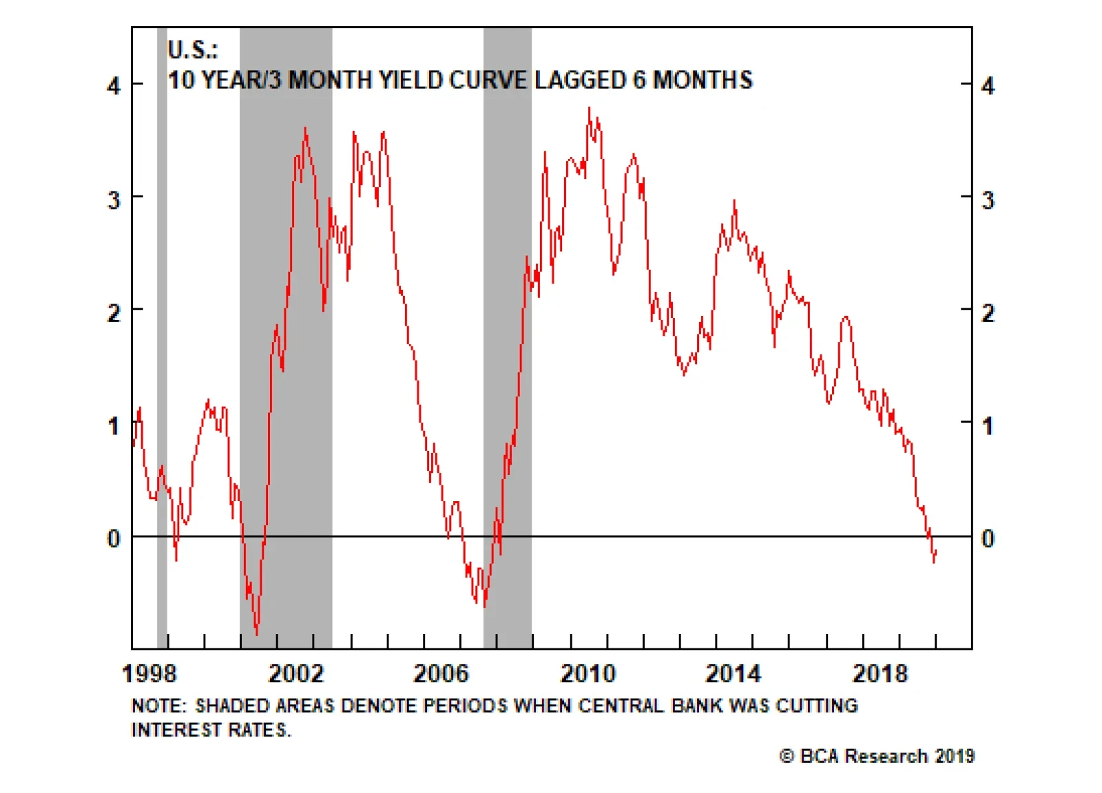
Highlights Chart 1Keep Tracking The CRB / Gold Ratio Keep Tracking The CRB / Gold Ratio Keep Tracking The CRB / Gold Ratio The Fed cut rates by 25 basis points last week, a move that Chairman Powell described as an “insurance” cut meant to counter the risks from trade tensions and global growth weakness. Powell also described the move as a “mid-cycle adjustment to policy” and not “the beginning of a lengthy cutting cycle”. We agree with the Fed’s “mid-cycle” view of the U.S. economy and think an extended cutting cycle is unwarranted, but the market clearly disagrees. Long-end yields fell on Powell’s remarks and fell further as U.S. / China trade tensions re-escalated during the past few days. The 2015/16 period continues to be a good roadmap for the current environment, and we expect the next big move in Treasury yields will be higher. The timing of that move, however, is highly uncertain. Our political strategists expect an increase in saber-rattling between the U.S. and China in the coming months, and bond yields will not rise until either trade tensions ease and/or the global growth data recover. We recommend a tactical neutral allocation to portfolio duration, but expect to switch back to below-benchmark when those conditions are met. The CRB / Gold ratio will continue to be a good guide for the 10-year yield (Chart 1). Feature Investment Grade: Overweight Chart 2Investment Grade Market Overview Investment Grade Market Overview Investment Grade Market Overview Investment grade corporate bonds outperformed the duration-equivalent Treasury index by 63 basis points in July, bringing year-to-date excess returns up to +432 bps. Corporate spreads widened somewhat following Jerome Powell’s perceived hawkishness at last week’s FOMC meeting, but that spread widening will prove fleeting. The Fed remains committed to keeping monetary policy accommodative and that means doing everything it can to prevent a significant tightening of financial conditions.1 The soaring price of gold is the strongest indicator of the Fed’s dovishness, and it is also a buy signal for corporate credit (Chart 2). In terms of valuation, Baa-rated securities offer the most value in investment grade corporate bond space. Baa spreads remain 7 bps above our cyclical target.2 Conversely, Aa and A-rated spreads are 3 bps and 4 bps below target, respectively (panel 4). Aaa spreads are 16 bps below target (not shown). The Fed’s Senior Loan Officer Survey for Q2, released yesterday, showed that commercial & industrial (C&I) lending standards eased for the second consecutive quarter. C&I loan demand continued to contract, but less aggressively than its recent pace (bottom panel). Easing lending standards usually coincide with spread tightening, and vice-versa.  Chart Chart High-Yield: Overweight Chart 3High-Yield Market Overview High-Yield Market Overview High-Yield Market Overview High-Yield outperformed the duration-equivalent Treasury index by 66 basis points in July, bringing year-to-date excess returns up to +673 bps. The average index option-adjusted spread tightened 6 bps in July, then widened 26 bps in the first two days of August. At 397 bps, it is currently well above the cycle-low of 303 bps. We see more potential for spread tightening in high-yield than in investment grade. Within investment grade, only Baa-rated spreads appear cheap. However, in high-yield, Ba-rated spreads are 71 bps above our target (Chart 3), B-rated spreads are 142 bps above our target (panel 3) and Caa-rated spreads are 298 bps above our target (not shown).3 Junk spreads also offer reasonable value relative to expected default losses. The current Moody’s baseline forecast calls for a default rate of 2.9% over the next 12 months, not far from our own projection.4 This would translate into 238 bps of excess spread in the High-Yield index, after adjusting for default losses (panel 4). This is comfortably above zero, and only just below the historical average of 250 bps. As noted on page 3, C&I lending standards have now eased for two consecutive quarters and job cut announcements are off their highs (bottom panel). Both trends are supportive of lower default expectations in the future. MBS: Neutral Chart 4MBS Market Overview MBS Market Overview MBS Market Overview Mortgage-Backed Securities outperformed the duration-equivalent Treasury index by 43 basis points in July, bringing year-to-date excess returns up to +32 bps. The conventional 30-year zero-volatility spread tightened 10 bps on the month, consisting of a 9 bps tightening in the option-adjusted spread (OAS) and a 1 bp decline in the compensation for prepayment risk (option cost). Falling mortgage rates hurt MBS in the first half of this year, as lower rates led to an increase in refi activity that drove MBS spreads wider (Chart 4). In fact, the conventional 30-year index OAS moved all the way back to its pre-crisis mean, before tightening last month (panel 3). However, as we noted in a recent report, the nominal 30-year MBS spread remains very tight, at close to one standard deviation below its historical mean.5 The mixed valuation picture means we are not yet inclined to augment MBS exposure, especially given the recent downleg in Treasury yields that could spur another small jump in refis. However, we are equally disinclined to downgrade MBS, given our view that Treasury yields are close to a trough. All in all, we expect the next big move in the MBS/Treasury basis will be a tightening, as global growth improves and mortgage rates rise. However, valuation is not sufficiently attractive to warrant more than a neutral allocation.   Government-Related: Underweight Chart 5Government-Related Market Overview Government-Related Market Overview Government-Related Market Overview The Government-Related index outperformed the duration-equivalent Treasury index by 30 basis points in July, bringing year-to-date excess returns up to +164 bps. Sovereign debt outperformed duration-equivalent Treasuries by 68 bps on the month, bringing year-to-date excess returns up to +490 bps. Local Authorities outperformed the Treasury benchmark by 31 bps, bringing year-to-date excess returns up to +244 bps. Meanwhile, Foreign Agencies outperformed by 49 bps, bringing year-to-date excess returns up to +153 bps. Domestic Agencies outperformed by 6 bps in July, bringing year-to-date excess returns up to +31 bps. Supranationals outperformed by 7 bps on the month, bringing year-to-date excess returns up to +36 bps. Sovereign debt remains very expensive relative to equivalently rated U.S. corporate credit (Chart 5). While the sector would benefit if the Fed’s dovish pivot eventually results in a weaker dollar, U.S. corporate bonds would still outperform in that scenario given the more attractive starting point for spreads. We continue to recommend an underweight allocation to Sovereigns. Unlike the debt of most other countries, Mexican sovereign bonds continue to trade cheap relative to U.S. corporates (bottom panel). While this remains an attractive option from a valuation perspective, the President’s on again/off again tariff threats make it a risky near-term proposition. Municipal Bonds: Neutral Chart 6Municipal Market Overview Municipal Market Overview Municipal Market Overview Municipal bonds outperformed the duration-equivalent Treasury index by 102 basis points in July, bringing year-to-date excess returns up to +58 bps (before adjusting for the tax advantage). The average Aaa-rated Municipal / Treasury yield ratio fell 8% in July, and currently sits at 78% (Chart 6). The ratio is more than one standard deviation below its post-crisis mean, and even below the 81% average that prevailed in the late stages of the previous cycle, between mid-2006 and mid-2007. We noted the strong outperformance of municipal bonds in our report two weeks ago, and recommended cutting exposure from overweight to neutral, based on how expensive the bonds have become.6 In that report we noted that Aaa-rated Municipal / Treasury yield ratios for 2-year, 5-year and 10-year maturities were all more than one standard deviation below average pre-crisis levels. Only 20-year and 30-year Aaa-rated municipal bonds continue to look cheap, and we recommend that investors focus muni exposure on that segment of the market. Fundamentally, state & local government balance sheets remain in decent shape and a material increase in ratings downgrades is unlikely any time soon (bottom panel). Our shift to a more cautious stance is driven purely by valuation, and not any immediate concern for municipal bond credit quality. Treasury Curve: Maintain A Barbell Curve Positioning Chart 7Treasury Yield Curve Overview Treasury Yield Curve Overview Treasury Yield Curve Overview The Treasury curve bear-flattened in July, before undergoing a roughly parallel shift down of about 30 bps in the first two days of August, following the FOMC meeting and news about the escalation of the U.S./China trade war. As we go to press, the 2/10 Treasury slope stands at 16 bps, 9 bps flatter than at the end of June. The 5/30 slope is currently 76 bps, exactly equal to its end-of-June level. Our 12-month Fed Funds Discounter is currently -78 bps (Chart 7). This means that the market is priced for roughly three more 25 basis point rate cuts during the next year. While we have shifted to a tactically neutral duration stance because of the uncertainty surrounding the timing of the next move higher in yields, three rate cuts on a 12-month horizon still seems excessive given the underlying strength of the U.S. economy. For this reason we are inclined to maintain a barbelled position across the Treasury curve, and also to stay short the February 2020 fed funds futures contract. The February 2020 contract is priced for three rate cuts spread over the next four FOMC meetings. A short position continues to make sense. On the yield curve, our butterfly spread models continue to show that barbells look cheap relative to bullets (see Appendix B). Further, the 5-year and 7-year yields will rise the most when the market prices-in a more hawkish path for the policy rate. Investors should favor the long-end and short-end of the curve, while avoiding the belly (5-year and 7-year). TIPS: Overweight Chart 8Inflation Compensation Inflation Compensation Inflation Compensation TIPS outperformed the duration-equivalent nominal Treasury index by 43 basis points in July, bringing year-to-date excess returns up to +71 bps. The 10-year TIPS breakeven inflation rate rose 8 bps in July to reach 1.77%, before falling back to 1.67% in the first few days of August (Chart 8). The 5-year/5-year forward TIPS breakeven inflation rate followed a similar path and currently sits at 1.88%. As we have noted in recent research, FOMC members are monitoring long-dated inflation expectations and are committed to keeping policy easy enough to “re-anchor” them at levels consistent with the Fed’s 2% target.7 In the long-run, this will support a return of long-dated TIPS breakeven inflation rates (both 10-year and 5-year/5-year forward) to our 2.3% - 2.5% target range. However, for breakevens to move higher, investors will also need to see evidence that realized inflation can be sustained near 2%. On that note, the core PCE deflator grew at an annualized rate of 2.48% during the past three months. However, the 12-month rate of change remains at 1.5%. The 12-month trimmed mean PCE inflation rate is currently running at 2%, exactly equal to the Fed’s target. In a recent report we noted that 12-month core PCE inflation has a track record of converging toward the trimmed mean.8 We see continued upside in core inflation over the remainder of the year, and therefore recommend an overweight allocation to TIPS versus nominal Treasuries.  ABS: Underweight Chart 9ABS Market Overview ABS Market Overview ABS Market Overview Asset-Backed Securities outperformed the duration-equivalent Treasury index by 8 basis points in July, bringing year-to-date excess returns up to +59 bps. The index option-adjusted spread for Aaa-rated ABS tightened 3 bps on the month. It currently sits at 31 bps, well below the pre-crisis mean of 64 bps (Chart 9). In addition to poor valuation, the sector’s credit fundamentals are shifting in a negative direction. Household interest payments continue to trend up, suggesting a higher delinquency rate going forward (panel 3). Meanwhile, the Fed’s Senior Loan Officer Survey for Q2, released yesterday, showed a continued tightening in lending standards for both credit cards and auto loans. Tighter lending standards usually coincide with rising delinquencies (bottom panel). On the bright side, stronger demand for both credit cards and auto loans was reported for the first time since the fourth quarter of 2016. All in all, the combination of poor value and deteriorating credit quality leads us to recommend an underweight allocation to consumer ABS.       Non-Agency CMBS: Neutral     Chart 10CMBS Market Overview CMBS Market Overview CMBS Market Overview Non-Agency Commercial Mortgage-Backed Securities outperformed the duration-equivalent Treasury index by 42 basis points in July, bringing year-to-date excess returns up to +234 bps. The index option-adjusted spread for non-agency Aaa-rated CMBS tightened 6 bps on the month. It currently sits at 64 bps, below average pre-crisis levels but above levels seen in 2018 (Chart 10). The macro outlook for commercial real estate looks somewhat unfavorable, with lenders tightening standards (panel 4) amidst falling demand (bottom panel). However, on a positive note, commercial real estate prices recently accelerated and are now much more consistent with current CMBS spreads (panel 3). Despite the mixed fundamental picture, CMBS still offer excellent compensation compared to other similarly-rated fixed income sectors.9 Agency CMBS: Overweight   Agency CMBS outperformed the duration-equivalent Treasury index by 26 bps in July, bringing year-to-date excess returns up to +119 bps. The index option-adjusted spread tightened 3 bps on the month and currently sits at 47 bps. The Excess Return Bond Map in Appendix C shows that Agency CMBS offer high potential return compared to other low-risk spread products. An overweight allocation to this defensive sector remains appropriate. Appendix A - The Golden Rule Of Bond Investing We follow a two-step process to formulate recommendations for bond portfolio duration. First, we determine the change in the federal funds rate that is priced into the yield curve for the next 12 months. Second, we decide – based on our assessments of the economy and Fed policy – whether the change in the fed funds rate will exceed or fall short of what is priced into the curve. Most of the time, a correct answer to this question leads to the appropriate duration call. We call this framework the Golden Rule Of Bond Investing, and we demonstrated its effectiveness in the U.S. Bond Strategy Special Report, “The Golden Rule Of Bond Investing”, dated July 24, 2018, available at usbs.bcaresearch.com. Chart 11 illustrates the Golden Rule’s track record by showing that the Bloomberg Barclays Treasury Master Index tends to outperform cash when rate hikes fall short of 12-month expectations, and vice-versa. Chart 11The Golden Rule's Track Record The Golden Rule's Track Record The Golden Rule's Track Record At present, the market is priced for 78 basis points of cuts during the next 12 months. We anticipate fewer rate cuts over that time horizon, and therefore anticipate that below-benchmark portfolio duration positions will profit. We can also use our Golden Rule framework to make 12-month total return and excess return forecasts for the Bloomberg Barclays Treasury index under different scenarios for the fed funds rate. Excess returns are relative to the Bloomberg Barclays Cash index. To forecast total returns we first calculate the 12-month fed funds rate surprise in each scenario by comparing the assumed change in the fed funds rate to the current value of our 12-month discounter. This rate hike surprise is then mapped to an expected change in the Treasury index yield using a regression based on the historical relationship between those two variables. Finally, we apply the expected change in index yield to the current characteristics (yield, duration and convexity) of the Treasury index to estimate total returns on a 12-month horizon. The below tables present those results, along with 95% confidence intervals. Excess returns are calculated by subtracting assumed cash returns in each scenario from our total return projections. Image Image Appendix B - Butterfly Strategy Valuation The following tables present the current read-outs from our butterfly spread models. We use these models to identify opportunities to take duration-neutral positions across the Treasury curve. The following two Special Reports explain the models in more detail: U.S. Bond Strategy Special Report, “Bullets, Barbells And Butterflies”, dated July 25, 2017, available at usbs.bcaresearch.com U.S. Bond Strategy Special Report, “More Bullets, Barbells And Butterflies”, dated May 15, 2018, available at usbs.bcaresearch.com Table 4 shows the raw residuals from each model. A positive value indicates that the bullet is cheap relative to the duration-matched barbell. A negative value indicates that the barbell is cheap relative to the bullet. Table 4Butterfly Strategy Valuation: Raw Residuals In Basis Points (As of August 2, 2019) Underinsured Underinsured Table 5 scales the raw residuals in Table 4 by their historical means and standard deviations. This facilitates comparison between the different butterfly spreads. Table 5Butterfly Strategy Valuation: Standardized Residuals (As of August 2, 2019) Underinsured Underinsured Table 6 flips the models on their heads. It shows the change in the slope between the two barbell maturities that must be realized during the next six months to make returns between the bullet and barbell equal. For example, a reading of +55 bps in the 5 over 2/10 cell means that we would only expect the 5-year to outperform the 2/10 if the 2/10 slope steepens by more than 55 bps during the next six months. Otherwise, we would expect the 2/10 barbell to outperform the 5-year bullet. Table 6Discounted Slope Change During Next 6 Months (BPs) Underinsured Underinsured Appendix C - Excess Return Bond Map The Excess Return Bond Map is used to assess the relative risk/reward trade-off between different sectors of the U.S. fixed income market. The Map employs volatility-adjusted breakeven spread analysis to show how likely it is that a given sector will earn/lose money during the subsequent 12 months. The Map does not incorporate any macroeconomic view. The horizontal axis of the Map shows the number of days of average spread widening required for each sector to lose 100 bps versus a position in duration-matched Treasuries. Sectors plotting further to the left require more days of average spread widening and are therefore less likely to see losses. The vertical axis shows the number of days of average spread tightening required for each sector to earn 100 bps in excess of duration-matched Treasuries. Sectors plotting further toward the top require fewer days of spread tightening and are therefore more likely to earn 100 bps of excess return. Chart 12   Ryan Swift, U.S. Bond Strategist rswift@bcaresearch.com Jeremie Peloso, Research Analyst jeremiep@bcaresearch.com Footnotes 1 Please see U.S. Bond Strategy / Global Fixed Income Strategy Weekly Report, “The Fed’s Got Your Back”, dated June 25, 2019, available at usbs.bcaresearch.com 2 For more details on how we arrive at our spread targets please see U.S. Bond Strategy Weekly Report, “The Value In Corporate Bonds”, dated February 19, 2019, available at usbs.bcaresearch.com 3 For more details on how we arrive at our spread targets please see U.S. Bond Strategy Weekly Report, “The Value In Corporate Bonds”, dated February 19, 2019, available at usbs.bcaresearch.com 4 Please see U.S. Bond Strategy Special Report, “Assessing Corporate Default Risk”, dated March 19, 2019, available at usbs.bcaresearch.com 5 Please see U.S. Bond Strategy Weekly Report, “The Long Awkward Middle Phase”, dated July 2, 2019, available at usbs.bcaresearch.com 6 Please see U.S. Bond Strategy Weekly Report, “A Message To The TIPS Market”, dated July 23, 2019, available at usbs.bcaresearch.com 7 Please see U.S. Bond Strategy Weekly Report, “A Message To The TIPS Market”, dated July 23, 2019, available at usbs.bcaresearch.com 8 Please see U.S. Bond Strategy Weekly Report, “Hedge Near-Term Credit Exposure”, dated May 28, 2019, available at usbs.bcaresearch.com 9 Please see U.S. Bond Strategy Weekly Report, “The Search For Aaa Spread”, dated March 12, 2019, available at usbs.bcaresearch.com Fixed Income Sector Performance Recommended Portfolio Specification Corporate Sector Relative Valuation And Recommended Allocation

Highlights Markets expressed disappointment over last week’s FOMC meeting, … : Equities sold off, Treasury yields slid, and the curve flattened. … but we didn’t think there was all that much to get excited about, … : Data dependence remains the Fed’s mantra, and it was never likely that the FOMC would signal that policy through September has been pre-programmed. … though the specter of escalating trade tensions was a bummer: We have followed our repeated exogenous-shock caveat with an acknowledgement of the gravity of trade barriers. Our geopolitical strategists don’t expect a resolution any time soon, though, and White House tweets are here to stay. Marginally easier monetary policy is not likely to have all that much of an effect on the economy: A reduction in the fed funds rate from 2.5% to 2% isn’t likely to turbo-charge housing or corporate investment, but we do expect that the major central banks’ easing bias will support risk assets. Feature The FOMC delivered the result we expected at the conclusion of its meeting last week: a 25-basis-point cut and a dovish adjustment to its balance sheet runoff plans. Markets acted as if they’d been blindsided. Apparently it really isn’t what you say, it’s how you say it. Or maybe, as our colleague Martin Barnes has long contended, press conferences and all the other assorted communications strategies do more harm than good. We have nearly reached the point of Fed fatigue ourselves, but there’s no ignoring the elephant in the room. The Fed is squarely in the center of every investor’s mind and may well remain there for the rest of what was shaping up as a slow-news month before the latest tariff move. American and Chinese negotiators have called it quits until September; lawmakers have left the building in London and Brussels; the ECB’s Governing Council will be idle until mid-September; and the winnowing of the Democratic field is so far off that even Bill de Blasio remains a presidential candidate. We devote this week’s report to an examination of increased accommodation’s implications for financial markets and the U.S. economy. What did the FOMC do on Wednesday? Chart 1An Adjustment, Not A New Direction An Adjustment, Not A New Direction An Adjustment, Not A New Direction The FOMC cut the fed funds rate by 25 basis points, to a range of 2-2.25%, and terminated its modest balance sheet reduction effort two months ahead of time. It studiously kept its options open with regard to future policy rate adjustments, with Chair Powell describing the cut as a “mid-cycle adjustment,” rather than a transition to full-on policy easing. The mid-cycle reference kiboshed hopes that the cut was meant to bring the curtain down on the tightening cycle that began at the end of 2015 (Chart 1). The hawkish surprise concerning the future direction of the fed funds rate overwhelmed the modestly dovish news that the Fed is immediately ending small-scale quantitative tightening. How did markets take the developments? Not so well, especially over the two hours of Wednesday afternoon trading following the decision. The S&P 500 sold off by close to 2% during the press conference, the dollar surged against the euro, and the yield curve flattened as long-dated Treasuries surged while the 2-year note sold off sharply. Equities recovered their losses in Thursday morning’s trading, though bonds and the dollar held much of their gains, before the latest salvo in the U.S.-China dispute sent investors in all markets scurrying for cover. Overall, financial markets were disappointed that they didn’t get a clearer signal that additional accommodation is on the way. Did markets overreact? In retrospect, it looks like they’d gotten their hopes up too high. The Fed wants to avoid surprises by keeping markets apprised of future developments, but it’s hard to envision it deliberately boxing itself in. It wants to preserve the flexibility to act as it sees fit, so data dependence remains the order of the day, just as it has for the last several years. We continue to take the Fed at its word that policy is not on a pre-set course. Markets seemed to be looking for a little more solicitousness from the Fed. Central bankers will presumably always attempt to guard their discretion, but the monetary policy path is far from clear, given elevated economic uncertainty. Between the stop-and-start trade hostilities with China and the Whack-a-Mole emergence of tariff threats against long-standing allies and trade partners, global manufacturing is reeling and corporate managers have every reason to hold back on capex. The differences of opinion within BCA reflect the lack of an obvious economic direction. Dissention within the Fed – Boston’s Rosengren and Kansas City’s George voted against last week’s cut, while Minneapolis’ Kashkari surely wanted it to be larger – shows that the way forward is not so clear-cut. So is it a good thing or a bad thing that the Fed cut rates? We view easier policy as a market positive over the one-year timeframe that drives most investors. There will come a point of diminishing returns, when risk assets no longer respond to incremental accommodation, but we don’t think we’re there yet. Equity multiples have room to expand before they become silly and the ECB is apparently preparing a new round of asset purchases. Given that it’s exhausted the supply of Eurozone sovereigns, it will have to proceed to evicting incumbent holders from their positions somewhat further out the risk curve, prodding them to venture out still further to redeploy the proceeds, putting downward pressure on spreads globally. How will a lower fed funds rate impact the economy? How much time do you have? The textbook answer is that a lower fed funds rate directly reduces the cost of financing big-ticket consumer purchases and corporate initiatives while indirectly nudging households and corporate managers to make them by boosting their confidence. Unconventional measures like asset purchases (QE) push investors further out the risk curve, lifting the prices of risky assets, lowering lending spreads and increasing asset holders’ wealth. They also promote a broader sense of well-being (the CNBC screen is framed in green, print headlines are cheerful, and jobs are increasingly easier to find), fueling confidence that helps reinforce the direct effects of easier policy. As Chair Powell put it in January, “Our policy works through changing financial conditions[,] … it’s … the essence of what we do.” The logic behind the textbook answer is undeniably sound, and it’s displayed in the simple six-channel model in Figure 1. People respond to incentives, and when the cost of consumption and investment falls, they are likely to save less and consume and invest more (Interest Rates/Substitution Effect). Increasing numbers of observers are becoming restless, however, as events on the ground don’t seem to jibe with the theory. Ten years of a negative real fed funds rate has failed to generate much oomph, and markets sputtered on cue once it tiptoed into positive territory (Chart 2), coinciding with the current global economic softness. Chart Chart 2Real Rates Are Still Low Relative To History Real Rates Are Still Low Relative To History Real Rates Are Still Low Relative To History Martin Barnes, our resident grumpy economist, scoffs at how little extraordinary accommodation has been able to achieve. (Don’t get him started on the communication strategies.) Even after adjusting for how a half-century of Scotland and Montreal weather has colored his perspective, he has a point. “Do you really want to buy equities and riskier bonds in an economy that needs this much help just to grow at 2%?” he might ask. For the time being, yes, we still do. Although the channels promoting economic activity are not functioning as reliably as they have in the past, the channels boosting asset prices – Portfolio Balance, Confidence/Risk Taking, and Interest Rates/Substitution – are still A-Okay (Figure 1). The initial reaction to the FOMC meeting suggests that it will be very hard for the Fed to surprise dovishly in a relative sense, blocking the Currency channel for the time being. The Credit channel is still hindered by post-crisis regulations from Basel to Capitol Hill, at least in terms of the official banking system. Trade tensions have roiled net exports via retaliatory tariffs and suppressed global aggregate demand.1 Shouldn’t housing be at the forefront of any pickup in activity? Chart 3Lower Rates Haven't Helped Much Yet Lower Rates Haven't Helped Much Yet Lower Rates Haven't Helped Much Yet Housing is the classic proxy for tracing the effects of easier policy on the domestic economy, since nearly all of its end consumers finance their purchases, and its domestic concentration insulates it from trade effects. It has failed to respond much to the monetary policy shifts that have brought 30-year fixed mortgage rates down nearly 100 basis points year to date (Chart 3). Fed skeptics suggest that the muted response is evidence of the declining efficacy of easy policy, though we have been inclined to read the data as an indication that homebuilders aren’t building enough starter and move-up homes to bring homeownership within reach of first-time homebuyers and median-income households. Housing should exhibit a high sensitivity to changes in monetary policy, but an abundance of other debt burdens and a lack of affordable supply may be holding it back.   One should have expected that the housing pickup would be muted, and slower to take hold in this expansion, given the severity of the recession and its mortgage-lending roots. Adjusted for inflation, private residential investment, which has declined slightly for four straight quarters, is just over two-thirds of its 2005 peak (Chart 4, middle panel). In the past, residential investment has been more sensitive to the level of the fed funds rate than its direction. Since 1961, the Fed has hiked rates in as many quarters as it has cut them, and the difference in annualized growth has been relatively modest: 2.8% when the Fed has been cutting rates, and 1.6% when it’s been raising them. Chart 4Residential Investment Responds To The Monetary Policy Backdrop... Residential Investment Responds To The Monetary Policy Backdrop... Residential Investment Responds To The Monetary Policy Backdrop... Per our equilibrium fed funds rate framework, we deem monetary policy to be accommodative when the fed funds rate is below our estimate of equilibrium, and restrictive when the funds rate exceeds it (Chart 4, top panel). Despite the fact that the Fed has hiked as often as it has cut since 1961, we estimate that policy has been easy for two-thirds of the time, and the difference in residential investment growth in the two policy states has been dramatic: 6.8% when policy is easy and -6.6% when policy is tight (Chart 4, bottom panel). With the Fed keeping policy easy for longer, housing will have the wind at its back, though it isn’t much more than a breeze at the moment. The same goes for construction employment, which has grown more rapidly under accommodative monetary policy (2.1% versus 0.7% when policy is tight), but has merely treaded water over the last 11 years of easy policy (Chart 5). Chart 5... And So Does Construction Employment ... And So Does Construction Employment ... And So Does Construction Employment The bottom line is that the jury is still out on housing activity. Low mortgage rates will help renters buy homes (and fill them with furniture and appliances), and put more cash in the pockets of homeowners who refinance their existing loans, but the market remains soft. Though it can’t be captured by the aggregate data, it does seem possible that median-income households may be burdened by too much student loan, automobile and/or credit card debt to save the required down payment.2 Disparities between households may well be holding the economy back, but they have a silver lining if they encourage the Fed to pursue accommodative policies for longer than it otherwise would. Will rate cuts give the economy a tangible lift? We don’t know for sure, but no one else does, either. We are convinced that easier monetary conditions will help the economy at the margin. Ten years into the expansion, though, it is not clear if the economy has pent-up demand that easier conditions will help release. Externally, worsening trade tensions could exacerbate the global manufacturing slowdown, further squeezing global aggregate demand, and exporting recession pressures to the U.S. Our mandate is not to forecast the economy in itself, though. We and our clients are investors, not government officials or public-policy professors, and we focus on the economy only to the extent that it impacts financial markets. In the near term, incremental accommodation should boost risk asset prices, provided that trade tensions don’t ratchet up enough to undermine investor, consumer and business confidence. Animal spirits matter, and if they shift decisively from greed and toward fear, they can become a self-fulfilling prophecy that sweeps monetary policy efforts before them. Ex-a significantly negative exogenous event, we remain constructive on the U.S. economy, and continue to look for a global revival outside of the U.S. Investment Implications The incremental information received this week – an FOMC meeting that mostly went off as we expected, a modest escalation in U.S. pressure on China in line with our geopolitical strategists’ warnings that a final deal is not at hand, mixed global manufacturing PMIs, a surge in U.S. consumer confidence, a straight-down-the-middle employment situation report, and an upward inflection in S&P 500 earnings growth that has 2Q EPS now tracking to a 2.7% year-over-year gain – did not change our perspective. We see U.S. economic growth decelerating from its 2018 pace, but remaining above trend, and an absence of imbalances that would make the economy more vulnerable. We have made our peace with recurring flare-ups of hostilities between the U.S. and China, and trade tensions will only change our investment outlook if they worsen materially. The Fed is not magic, but it is doing the best it can to keep the expansion going for the purpose of spreading its gains as broadly as possible, and the easing bias among major central banks is gathering force. On balance, the new information received last week didn’t do anything to change our overall take. We remain constructive, and think investment portfolios should as well. We recognize that the climate is uncertain, and that we should accordingly dial back our conviction. Part of the reason the agency mortgage REITs appeal to us at this juncture is that they offer the opportunity to reduce equity beta and enhance a balanced portfolio’s capacity to absorb shocks. We watched the flattening in the yield curve with dismay, but we continue to expect that incremental monetary accommodation will promote a steeper curve. Easier monetary conditions promote growth, boosting the real component of interest rates, and can stoke inflation pressures when an economy is operating at or above capacity, as the U.S. has been for over a year. We remain vigilant, but our base-case constructive take is unchanged.   Doug Peta, CFA Chief U.S. Investment Strategist dougp@bcaresearch.com Footnotes 1 As we were preparing to go to press on Thursday, the U.S. announced the imposition of new tariff levies on the subset of Chinese imports that hadn’t yet been subjected to tariffs. The move supported our geopolitical strategists’ view that the trade war is unlikely to be settled soon. 2 Andriotis, AnnaMaria; Brown, Ken; and Shifflett, Shane, “Families Go Deep in Debt to Stay in the Middle Class,” Wall Street Journal, August 1, 2019.

Double Trouble Double Trouble S&P Materials (Neutral) Downgraded from Overweight S&P Chemicals (Underweight) Downgraded from Neutral Besides being exposed to the toxic U.S. manufacturing data, S&P chemicals are also taking a hit from the global economic slowdown as nearly 60% of sector revenues are coming from abroad. Falling U.S. chemical exports and the resulting buildup in inventories spell trouble for the industry (second & third panels). Consequently, we warranted a below benchmark allocation to the S&P chemicals index in our May 21st  Weekly Report as global macro headwinds will continue to weigh on this deep cyclical sub-index. Given that chemicals have a 74% market cap weight in the S&P materials index, our move to go underweight on the sub-index level also pushed the entire S&P materials index from overweight to neutral. Bottom Line: Continue avoiding deep cyclical sectors and remain defensive. For the full summary of our recent moves, please see this Monday’s Weekly Report.  

Stick With The U.S. Consumer Stick With The U.S. Consumer S&P Hypermarkets (Overweight) Upgraded from Neutral S&P Soft Drinks (Neutral) Upgraded from Underweight As a follow up to our yesterday’s Insight where we outlined some of our reasons to go underweight the S&P technology sector, today we focus on two defensive sub-sectors that will benefit from the spreading cracks in the U.S. economy: S&P hypermarkets and S&P soft drinks. Both sub-sectors enjoy deteriorating macroeconomic conditions, which are currently reflected in the steep fall in U.S. economic data surprises, the drubbing of the 10-year U.S. treasury yield, melting inflation and rapidly contracting ISM PMI numbers (see chart) Bottom Line: Stick with defensive consumer stocks. For a more detailed discussion on S&P hypermarkets and S&P soft drinks, please see our July 15 Weekly Report and “Bubbling Up” Insights,1 respectively. For the complete list of our recent moves, please see our Monday’s Weekly Report. ​​​​​​​   1      Please see BCA U.S. Equity Strategy Insight Reports, “Bubbling Up (Part I)” and “Bubbling Up (Part II)”, dated July 24, 2019 available at uses.bcaresearch.com.

Highlights China’s infrastructure investment growth rate could rebound moderately from its current nominal 3% pace, but will remain well below the double-digit rate it has registered for most of the past decade.  A lack of funding for local governments and their financing vehicles will somewhat cap the upside in infrastructure fixed-asset investment (FAI) in the next six to nine months. Special bond issuance will be insufficient to ensuring a major recovery in infrastructure spending. Investors should tread cautiously on infrastructure plays in financial markets. Feature Chart I-1Chinese Infrastructure Investment: Double-Digit Growth Again? Chinese Infrastructure Investment: Double-Digit Growth Again? Chinese Infrastructure Investment: Double-Digit Growth Again? Nominal infrastructure investment growth in China has slowed from over 15% in 2017 to 3% currently (Chart I-1). This is the weakest growth rate since 2005 excluding the late 2011-early 2012 period. Over the past decade, each time the Chinese economy experienced a considerable slowdown, infrastructure construction was ramped up to revive growth. Infrastructure spending growth skyrocketed in 2009 and was also boosted in 2012. In 2015-2016, it was not allowed to decelerate with the issuance of nearly RMB 2 trillion of special infrastructure bonds. This time the government has also reacted. Since mid-2018, the Chinese authorities have dramatically raised local governments’ special bonds balance limits, prompted local governments to front-load their issuance this year, and also encouraged the private sector to participate in public-private partnership (PPP) infrastructure projects. Will Chinese infrastructure FAI growth accelerate over the next six to nine months from its current nominal 3% pace to double digits? The short answer is no. Chart I-2 We believe Chinese infrastructure investment growth could rebound moderately in the next six to nine months, but will still remain below the double-digit growth seen in the past and well below the 18% average growth of the past 15 years. For purposes of this report, the composition of “infrastructure” includes three categories – (1) Transport, Storage and Postal Service, (2) Water Conservancy, Environment & Utility Management, and (3) Electricity, Gas & Water Production and Supply. Chart I-2 presents the breakdown of the nominal infrastructure FAI by category. Funding Constraint Preceding both the 2011-2012 and 2018 infrastructure investment slumps, the Chinese central government increased its scrutiny on local government debt and tightened funding conditions for infrastructure projects. As a result, all three categories of infrastructure spending experienced a sharp deceleration (Chart I-3). Overall, financing and qualitative limitations that Beijing imposes on local government infrastructure spending hold the key to the outlook. We believe Chinese infrastructure investment growth could rebound moderately in the next six to nine months, but will still remain below the double-digit growth seen in the past and well below the 18% average growth of the past 15 years. Looking forward, without a considerable recovery in available financing, there will be no meaningful rebound in Chinese infrastructure investment and construction activity. For now, we are not very optimistic on financing. Chart I-4 shows the breakdown of the major funding sources of Chinese infrastructure investment. All of them are likely to face considerable funding constraints over the next six to nine months. Chart I-3Chinese Infrastructure Investment Growth Has Decelerated Across The Board Chinese Infrastructure Investment Growth Has Decelerated Across The Board Chinese Infrastructure Investment Growth Has Decelerated Across The Board Chart I-4   1. Self-Raised Funds Self-raised funds contribute nearly 60% of overall infrastructure funding. They include net local government special bond issuance, PPP financing and government-managed funds’ (GMFs) revenues excluding proceeds from special bond issuance. A. Local government special bond issuance, which is exclusively used to fund infrastructure projects, has been the major source of financing for local governments in the past 12 months. The authorities significantly boosted net local government bond issuance to RMB 1.2 trillion in the first six months of this year from only RMB 361 billion in the same period in 2018. However, the amount of special bond issuance in the second half of this year will unlikely be significant enough to boost infrastructure FAI greatly. First, the central government has not only set a limit on the aggregate local government special bond balance, but it also set limits for each of the 31 provinces/provincial-level cities.1 In the past three years, nearly all provinces did not use up their special bond issuance quotas. This resulted in an outstanding aggregate amount of special bonds of only about 85% of the limit.2 In both 2017 and 2018, local governments were left with RMB 1.1 trillion special bond issuance quota unused for that year. Second, based on the limit on outstanding amount special bonds set by the central government for the end of 2019, local governments could issue another RMB 0.8-1 trillion of special bonds in the second half of this year. In comparison, in 2018, the issuance was heavily concentrated in the second half of the year with RMB 1.6 trillion. Our estimate shows there will be only RMB 400-600 billion increase in net total special bond issuance in 2019 versus 2018.3 This will translate into a merely 2-3% growth in Chinese infrastructure investment. Third, net local government special bond issuance made up only 15% of overall infrastructure FAI over the past 12 months. Hence, there is still a huge financing gap to be filled (Chart I-5). B. Public-private partnerships (PPP) are unlikely to meet the financing shortage either. PPPs have become an important financing model for Chinese local governments to fund infrastructure investments since 2014. Nevertheless, to control rising local government debt risks, the central government has tightened regulations on PPP projects since early last year. A series of tightened rules have resulted in a sharp deceleration in both PPP investment and overall infrastructure investment growth. Consequently, PPPs contributions to total infrastructure FAI have plunged from over 30% in 2017 to 10% currently (Chart I-6). Chart I-5Special Bond Issuance Accounted For Only 15% Of Infrastructure FAI Special Bond Issuance Accounted For Only 15% Of Infrastructure FAI Special Bond Issuance Accounted For Only 15% Of Infrastructure FAI Chart I-6Public-Private Partnerships: Too Small To Meet The Financing Shortage Public-Private Partnerships: Too Small To Meet The Financing Shortage Public-Private Partnerships: Too Small To Meet The Financing Shortage   So far, the rules on PPP projects on local governments remain tight. In March, the central government tightened its rule on local government participation in PPP projects. The new rule states that, if a local government has already spent more than 5% of its overall general expenditures on PPP projects excluding sewage and waste disposal PPP projects, it will not be allowed to invest in any new PPP projects. Before March, the threshold was over 10%. In early July, the National Development and Reform Commission (NDRC) demanded all PPP projects undertake a thorough feasibility study. The NDRC emphasized that PPP projects that do not follow standard procedures will not be allowed. Chart I-7Government-Managed Funds: Headwinds From Falling Land Sales Government-Managed Funds: Headwinds From Falling Land Sales Government-Managed Funds: Headwinds From Falling Land Sales C. Government-managed funds (GMF) excluding special bond issuance accounts, which contribute about 15% of overall infrastructure financing, are also facing constraints. According to the country’s Budget Law, the GMF budget refers to the budget for revenues and expenditures of the funds raised for specific developmental objectives. In brief, GMFs constitute de-facto off-balance-sheet government revenues and spending. Land sales by local governments are one major revenue source for GMFs. Contracting property floor space sold is likely to depress real estate developers’ land purchases, further reducing local governments’ revenues from selling land (Chart I-7). This will curb local governments’ ability to finance their infrastructure projects through GMFs. 2. Domestic Loans Domestic loans contribute to about 15% of overall infrastructure financing. Infrastructure projects are generally long term in nature. Presently, the impulse of non-household medium- and long-term (MLT) lending has stabilized but has not yet improved (Chart I-8). While not all of MLT loans are used for infrastructure, sluggish MLT lending reflects commercial banks’ reluctance to finance infrastructure projects. We believe a decelerating economy, mounting local government debt, and often-low returns on infrastructure projects will continue to constrain loan funding of infrastructure projects from both banks and the private sector. 3. General Government Budget The general government budget (which includes central and local governments) accounts for about 15% of overall infrastructure financing. The general budget is also facing headwinds from declining revenue due to recent tax cuts and lower corporate profit growth (Chart I-9). Chart I-8Sluggish Medium/Long-Term Bank Lending Sluggish Medium/Long-Term Bank Lending Sluggish Medium/Long-Term Bank Lending Chart I-9Government General Budget: Large Deficit Government General Budget: Large Deficit Government General Budget: Large Deficit   Bottom Line: Funding constraints will likely linger, making any recovery in Chinese infrastructure investment growth moderate over the next six to nine months. Local government special bonds will not be a game-changer. Their net issuance accounted for only 15% of overall infrastructure FAI over the past 12 months. While local governments could issue another RMB 0.8-1 trillion of special bonds in the second half of 2019, it would be well below the RMB 1.4 trillion of special bond issuance that was rolled out in the second half of 2018. FAI In Transportation: In Nominal Terms… The transportation sector accounts for about 31% of total Chinese infrastructure investment. It includes railway, highway, urban public transit, air and water transport. Table I-1 shows the 13th five-year (2016-2020) transportation investment plan released by the government in February 2017,4 which excludes urban public transit. Chart I- The authorities planned to invest RMB 15 trillion in the transportation sector over the five-year period between 2016 and 2020, with highways accounting for over half of the investment, followed by railways (23%), air transportation (4.3%) and water transportation (3.3%). The table also shows our calculation of the realized investment amount in these four sub-sectors for the period of January 2016 to June 2019. Local government special bonds will not be a game-changer. Their net issuance accounted for only 15% of overall infrastructure FAI over the past 12 months. Table I-1 suggests the remaining FAI for the transportation sector for the July 2019 to December 2020 period will be considerably smaller than the FAI amount over the past 18 months. This entails a major drag on infrastructure investment at least over the next 18 months. It is important to emphasize that this is conditional on the central planners in Beijing sticking to their five-year plan for infrastructure FAI. As of now, there has been no announcement of revisions to these five-year FAI targets. Bottom Line: China has already completed the overwhelming majority of its planned transportation FAI for 2016-2020. Consequently, without revisions to the targets and budgets by central planners in Beijing, transportation investment will likely contract year-on-year over the next 18 months. …And Real Terms Table I-2 summarizes the 2020 targets for major Chinese infrastructure development (urban rail transit, railway, highway and airport) in real terms. Chart I- Chart I-10Transportation 2020 Targets: Not Far Away Transportation 2020 Targets: Not Far Away Transportation 2020 Targets: Not Far Away In real terms, the annual growth of transportation infrastructure will likely be 4.2% in both 2019 and 2020. We illustrated in the previous section that the five-year budget plan had been front-loaded, leaving a very small budget for transportation investment over the next 18 months. This may suggest that without considerably exceeding the budget, transportation infrastructure will fail to achieve the 4.2% annual growth in real terms both this year and next. In brief, more funding should be dispatched/allowed by the central planners in Beijing for infrastructure FAI not to shrink. Second, urban rail transit, high-speed railways, highways and airports will reach their respective 2020 targets, while non-high-speed railway construction will likely be a little bit off its 2020 target. Third, based on the 2020 targets, urban rail transit will enjoy very fast growth over the next one and a half years. Fourth, the growth of high-speed railways and highways will be very low, at around 1-2% in real terms (Chart I-10). Finally, while the number of airports will increase at a faster pace, their contribution to overall infrastructure investment will remain insignificant as they only account for about 1.4% of overall infrastructure investment. Bottom Line: In real terms, transport infrastructure growth will likely be only about 4% over the next six to nine months. Future Infrastructure Investment Focus Urban rail transit, environmental management and public utility management will likely be the major driving forces for Chinese infrastructure investment over the next 18 months. Urban rail transit line length will likely register fast growth of around 10% over the next six to nine months. As the central government enforces increasingly stringent rules on environmental protection, investment in environmental management will likely experience continued growth acceleration (Chart I-11). China has already completed the overwhelming majority of its planned transportation FAI for 2016-2020. Consequently, without revisions to the targets and budgets by central planners in Beijing, transportation investment will likely contract year-on-year over the next 18 months. Meanwhile, as the country’s urbanization continues and more townships and city suburbs become urbanized,5 public utility management investment will also grow moderately. Public utility management investment, contributing a massive 45% of overall infrastructure investment, includes sewer systems, sewer treatment facilities, waste treatment and disposal, streetlights, city roads construction, parks, bridges and tunnels in the city. Investment Implications Investors should not hold their breath expecting a major upswing in infrastructure FAI and a major rally in related financial markets. Chinese steel demand is sensitive to construction of railways and urban rail transit lines (Chart I-12, top panel). In turn, mainland cement demand is dependent on highway construction (Chart I-12, bottom panel). Chart I-11Environment Management: Will Continue Booming Environment Management: Will Continue Booming Environment Management: Will Continue Booming Chart I-12Chinese Infrastructure Spending Will Moderately Boost Steel & Cement Demand... Chinese Infrastructure Spending Will Moderately Boost Steel & Cement Demand... Chinese Infrastructure Spending Will Moderately Boost Steel & Cement Demand...   Chart I-13...And Steel & Cement Prices At The Margin ...And Steel & Cement Prices At The Margin ...And Steel & Cement Prices At The Margin The infrastructure sector accounts for about 10-15% of total Chinese steel use, and about 30-40% of Chinese cement consumption. Nevertheless, given that we believe Chinese infrastructure spending will only have a moderate recovery, the positive effect on steel and cement prices will be muted as well (Chart I-13). The same holds true for spending on industrial machinery, equipment, chemicals and various materials. Notably, risks to this baseline scenario of a muted recovery are to the downside because of the lack of funding. Barring a substantial increase in the special bond issuance quota this year or a major credit binge, infrastructure FAI growth could in fact stall. Ellen JingYuan He, Associate Vice President ellenj@bcaresearch.com   Footnotes 1  Please note that the central government only set the special bond balance limit (not the quota) for local governments. The often-cited “quota” in the news is derived by calculating the difference between the current limit and the previous year’s limit. The “quota” used in this report is the difference between the current special bond balance limit and the actual special bond balance of the previous year end. 2  At the end of 2018, Chinese special bond balance was RMB 7.4 trillion, only 85.8% of the special bond balance limit of RMB 8.6 trillion. This ratio was 84.6% in 2017 and 85.5% in 2016. On average, the ratio was 85.3% in the past three years. 3  Given that the central government is aiming to somewhat stimulate infrastructure spending by increasing special bond issuance, we assume special bond balance at the end of 2019 to reach 88%-90% of the limit (RMB 10.8 trillion) that it has set for 2019. This will be higher than the 85% average of the past three years. In turn, this means that the special bond balance at the end of this year will likely be RMB 9.5-9.7 trillion. Since the balance at the end of last year was RMB 7.4 trillion, this results that net special bond issuance will be around RMB 2.1-2.3 trillion in 2019. Given the net special bond issuance last year was RMB 1.7 trillion, it follows that there will only be a RMB 400-600 billion increase in total special bond issuance in 2019 versus 2018. 4  Please see www.gov.cn/xinwen/2017-02/28/content_5171576.htm, published February 28, 2017, by the Chinese central government website. 5  Please see Emerging Markets Strategy/China Investment Strategy Special Report “Industrialization-Driven Urbanization In China Is Losing Steam,” dated January 2, 2019, available on ems.bcaresearch.com

Feature GAA DM Equity Country Allocation Model Update Chart 1GAA DM Model Vs. MSCI World GAA DM Model Vs. MSCI World GAA DM Model Vs. MSCI World The GAA DM Equity Country Allocation model is updated as of July 31, 2019.  The quant model reversed its abnormal upgrade of Sweden in the previous model update. In hindsight, the model’s behavior when a bond yield moves close to zero needs to be watched closely. Currently, the model still favors Spain, Italy, Germany, Netherland and Australia at the expenses of U.S., Japan, U.K., France and Canada, as shown in Table 1.  As shown in Table 2 and Charts 1, 2 and 3, the overall model underperformed the MSCI World benchmark by 94 bps in July, largely driven by 146 bps of underperformance from the Level 2 model, and 26 bps of underperformance from the Level 1. Directionally, 7 out of the 12 choices generated positive alpha. However, the overweight in Sweden and Spain generated outsized underperformance. Since going live, the overall model has outperformed by 94 bps, with 297 bps of outperformance by the Level 2 model, offset by 42 bps of underperformance from the Level 1. Table 1Model Allocation Vs. Benchmark Weights GAA Quant Model Updates GAA Quant Model Updates Table 2Performance (Total Returns In USD %) GAA Quant Model Updates GAA Quant Model Updates Chart 2GAA U.S. Vs. Non U.S. Model (Level 1) GAA U.S. Vs. Non U.S. Model (Level 1) GAA U.S. Vs. Non U.S. Model (Level 1) Chart 3GAA Non U.S. Model (Level 2) GAA Non U.S. Model (Level 2) GAA Non U.S. Model (Level 2)   Please see also the website http://gaa.bcaresearch.com/trades/allocation_performance. For more details on the models, please see Special Report, “Global Equity Allocation: Introducing The Developed Markets Country Allocation Model,” dated January 29, 2016, available at https://gaa.bcaresearch.com. Please note that the overall country and sector recommendations published in our Monthly Portfolio Update and Quarterly Portfolio Outlook use the results of these quantitative models as one input, but do not stick slavishly to them. We believe that models are a useful check, but structural changes and unquantifiable factors need to be considered too in making overall recommendations. GAA Equity Sector Selection Model The GAA Equity Sector Model (Chart 4) is updated as of July 31, 2019. Chart 4Overall Model Performance Overall Model Performance Overall Model Performance The model’s tilts between cyclicals and defensives have changed compared to last month. Following the Fed’s decision to cut interest rates yesterday, the liquidity component shifted its inputs to phase 4 – a period in which the central bank is cutting rates, while simulative monetary conditions persist. Although this should favor most cyclical sectors, the lack of evidence of global growth bottoming is tilting the model to favor a mixed bag of sectors. The valuation component continues to remain muted across all sectors. The model is now overweight 4 sectors in total, 2 cyclical and 2 defensive sectors. These are Consumer Discretionary, Information Technology, Consumer Staples, and Healthcare. Table 3Model’s Performance (March 1, 2019 - Current) GAA Quant Model Updates GAA Quant Model Updates Table 4Current Model Allocations GAA Quant Model Updates GAA Quant Model Updates   For more details on the model, please see the Special Report “Introducing the GAA Equity Sector Selection Model,” dated July 27, 2016, as well as the Sector Selection Model section in the Special Alert “GAA Quant Model Updates,” dated March 1, 2019 available at https://gaa.bcaresearch.com. Xiaoli Tang, Associate Vice President xiaoliT@bcaresearch.com Amr Hanafy, Research Associate amrh@bcaresearch.com Footnotes

Continue Playing Defense Continue Playing Defense Neutral Downgrade Alert This Monday we published a summary of our portfolio allocation changes that we made over the past couple of months. They key underlying theme running through most of our recent moves was to reduce our cyclical exposure and pocket in some profits. Today we highlight one of the major moves we are preparing to make: downgrade the S&P technology sector. The downgrade will be executed via the S&P software index. As a reminder, we have a stop at the 27% relative return mark and once it’s triggered, we will go neutral on software pushing the overall tech sector to a below benchmark allocation. Our EPS model for the overall tech sector is on the verge of contraction on the back of sinking capex and a seemingly invincible U.S. dollar (middle panel). The San Francisco Fed’s Tech Pulse Index is also closing in on the expansion/contraction line warning that tech stocks are in for a rough ride (bottom panel). Bottom Line: We reiterate our defensive stance on the U.S. equity market as the risk/reward remains to the downside. For the full summary of our recent moves, please see this Monday’s Weekly Report.  

Highlights A decade after the financial crisis, yield remains scarce: The global count of bonds trading at negative yields seems to grow every week, squeezing a broad swath of investors who are desperate for coupon income. Increasingly accommodative monetary policy is not on income investors’ side, … : Dovish pivots from the Fed and the ECB ensure that low-to-negative yields won’t go away soon. … but it is quite friendly for maturity transformation strategies in the near term: Borrowing short to lend long is far from a fail-safe strategy, but it should dovetail nicely with reflationary Fed policy for at least the rest of the year. The time is ripe for returning to the agency mortgage REITs: Among public securities, agency mortgage REITs offer the most direct exposure to maturity transformation. Feature Economic data and corporate earnings releases remain mixed enough to provide both bulls and bears with ample support for their leanings. The debate within BCA remains spirited, and is emblematic of the debate among investors. Per the financial media, it seems as if the scolds are getting the most attention,1 even as the S&P 500 keeps setting new highs. One thing that both camps agree on, however, is that nothing is cheap. Equities are not terribly expensive, but bonds appear to have little chance of matching their historical return profile. Investors seeking income, from individuals and advisors, to pension funds, life insurers and endowments needing to meet a fixed schedule of liabilities, are under siege a decade into ZIRP and NIRP. With rate cuts on the horizon in the U.S., and the ECB preparing to ramp up accommodation, the pressure on income-seeking investors to throw caution to the wind and ignore credit quality shows no sign of abating. Maturity transformation – borrowing short to lend long – fits the Fed’s reflationary goals like a glove, and offers an alternative to abandoning credit standards. Contrary to popular belief, banks no longer pursue maturity transformation. Chastened by the savings-and-loans’ demise in the ‘80s, they make heavy use of swaps to keep a tight rein on asset-liability mismatches. Maturity transformation is agency mortgage REITs’ raison d’être, however, and aside from some hedging to ensure survival in the face of adverse interest-rate moves, they actively embrace it. The Agency mREIT Formula Mortgage REITs (“mREITs”) finance real estate investment, either by lending directly to property owners or by purchasing mortgages and/or mortgage-backed securities (“MBS”). Agency mREITs invest solely or predominantly in instruments issued or guaranteed by Fannie Mae, Freddie Mac or Ginnie Mae. MBS issued by these entities are explicitly backed by the full faith and credit of the United States and bear little to no credit risk. The agency mortgage REITs stumbled ahead of all four of the yield curve inversions they’ve experienced, and six years of flattening has ground down their share prices. Despite the negligible credit risk in their investment portfolios, agency mREITs themselves are far from riskless – leveraged carry trading strategies are not for the faint of heart – but they have performed much better than non-agency mREITs, some of which go bust in every cycle. The agency mREITs are a much purer play on the term structure of rates than their non-agency peers. Their borrow-short-to-lend-long model is intentionally designed to exploit the yield curve’s typical upward slope. Though they stumble ahead of inversions (Chart 1), they are an attractive portfolio component when the fed funds rate outlook is benign and the curve is poised to steepen. Chart 1The Steeper The Better The Steeper The Better The Steeper The Better Banks are happy to lend against pristine collateral for short timeframes, allowing agency mREITs to build RMBS portfolios 10 times the size of their equity capital. Figure 1 illustrates the mechanics of building an agency mREIT portfolio. A new mREIT first raises equity in a public offering and uses the proceeds to purchase a portfolio of agency-backed residential MBS (“agency RMBS”). It then uses the portfolio as collateral for a secured repurchase (“repo”) loan, typically with a 30-, 60- or 90-day term, the proceeds of which it recycles into more agency RMBS.  With banks and brokers lending 95 cents on the dollar against agency collateral, an agency mREIT can easily amass asset portfolios several times the value of its equity capital. As long as portfolio income exceeds the sum of repo interest and operating expenses, it will be profitable. Chart Table 1 lists all of the constituents of our Agency Mortgage REIT Index since its 1998 inception, along with the current constituents’ price-to-book multiples, dividend yields, betas versus the S&P 500 and leverage ratios. As a group, the agency mREITs have high dividend yields, low equity betas and considerable leverage. 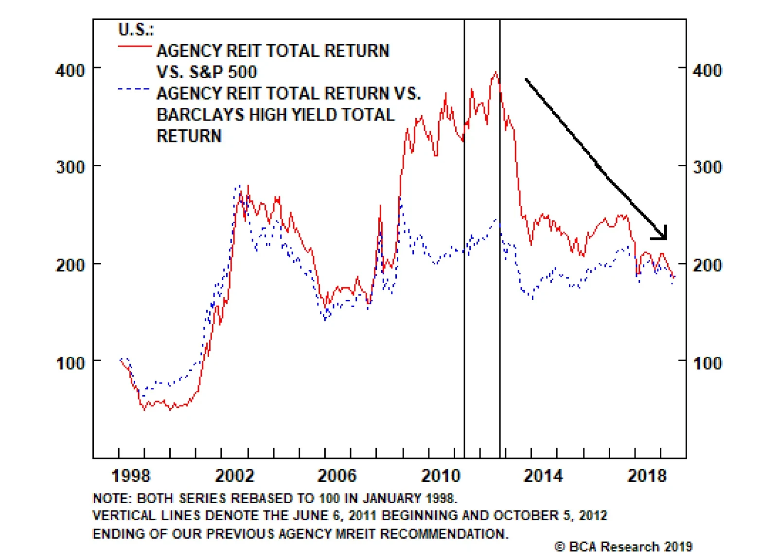Table 1Agency Mortgage REIT Index Constituents Agency Mortgage REITs Are Back In Season Agency Mortgage REITs Are Back In Season Low beta and high leverage could be a nice mix when the economy is mushy and the Fed and other major central banks are ramping up accommodation. Then And Now The last time we recommended the agency mREITs (June 2011 through September 2012), they handily outperformed the S&P 500 and the Bloomberg Barclays High Yield Index on a total return basis (Chart 2). Uninspiring growth and easy monetary policy proved to be a potent mix for agency mREIT outperformance. The backdrop looks similar to us now, and we expect that the agency mREITs will outdistance high-yield corporate bonds over the rest of the year. They may be hard-pressed to top the S&P 500 under more constructive economic and market scenarios, but they should help protect other equity exposures in the event that economic growth and equities slump. Chart 2The Agency Mortgage REITs Boosted Our Returns In 2011-12, ... The Agency Mortgage REITs Boosted Our Returns In 2011-12, ... The Agency Mortgage REITs Boosted Our Returns In 2011-12, ... The Incredible Shrinking Stock Price Agency mREITs trade on their price-to-book multiples, but REIT rules leave the companies with little chance to grow book value. REITs have to distribute 90% of their annual income to shareholders to maintain their tax-preferred status, and they pay no income tax at the corporate level if they distribute all of it. The upshot is that mREITs have no retained earnings, which stymies them from growing book value.   In exchange for optimal tax efficiency, REITs give up the potential to compound their way to growth. Chart 3...But They've Run Into Headwinds Since ...But They've Run Into Headwinds Since ...But They've Run Into Headwinds Since Price-to-book multiples swung wildly in the group’s first decade, but have settled into a tight post-crisis range (Chart 3). If book value can’t grow, and multiples are capped around 1, stock price appreciation is unlikely to contribute to total returns. History suggests that investors should actually expect some modest drag from capital losses; all but one of the stocks in our Agency mREIT Index have declined since their inclusion2 (Chart 4). The drag follows from the constraints of the REIT rules; companies that can’t retain earnings and have already reached their borrowing capacity can only grow by issuing stock, but companies only receive about 95% of the proceeds from offerings after underwriting fees.3 The practical takeaway is that the agency mREITs are not a through-the-cycle play, and investors should only add them to their portfolios when they are comfortable that price declines are not likely to undermine dividend distributions. Chart 4 Honey, I Shrunk The Share Price. Agency mREIT Vulnerabilities The agency mREIT model has three inherent vulnerabilities: it relies on maturity transformation, it employs copious amounts of leverage, and it has convexity working against it. None is likely to prove fatal for entities that are reasonably prudent about hedging rate exposures, limiting leverage, and guarding against prepayments, but double-digit annual returns are not pre-ordained. Each management team makes its own hedging choices, but all agency mREITs maintain considerable duration mismatches. Unexpected changes in the term structure of rates have the potential to upend shareholder returns. Chart 5Repo Funding Is Reliable Repo Funding Is Reliable Repo Funding Is Reliable Our index constituents have a considerable amount of leverage. With 5-cent haircuts on agency repo financing, mREITs can theoretically build an agency MBS portfolio equivalent to 20 times the value of its equity capital. Maximal leverage would leave very little room to maneuver under duress, but leverage around ten times has not historically posed a problem. Given that agency MBS is gilt-edged collateral, we expect that the agency mREITs will be able to roll over their repo financings in a stress scenario, just as they were able to amidst the crisis (Chart 5). Interest rate volatility is also a headwind, independent of the level of rates. Under standard U.S. mortgage terms, MBS investors implicitly grant options to borrowers by allowing them the unlimited right to prepay their obligations without penalty (see Box). Options increase in value as the volatility of their underlying reference asset increases, so MBS values move inversely with changes in interest rate volatility. The good news for the mREITs is that increasingly accommodative Fed and ECB policy should act to tamp down rate volatility in the near term. The agency mREIT model proved its resiliency at the height of the crisis. Even in times of peak stress, it’s possible to borrow against the best collateral.   Box An Equity Investor’s Guide To Negative Convexity Even for fixed income lifers, mortgages can be a dauntingly complex product, largely because of borrowers’ ability to prepay their loans, without penalty, at any time.  This prepayment option gives mortgages and MBS what fixed income professionals call “negative convexity.” Long-duration, non-callable bonds are said to be positively convex.  That is, their value increases at an increasing rate as interest rates fall and decreases at a decreasing rate as interest rates rise.  Mortgage borrowers’ prepayment option prevents mortgage lenders from enjoying the full effect of convexity because the more the present value of a mortgage’s future payment stream rises as rates fall, the less likely lenders will realize it as savvy borrowers refinance into one offering a lower interest rate. This effect is called negative convexity and it is why mortgage investors must be compensated with higher yields.  Fannie, Freddie and Ginnie securities therefore yield more than Treasuries, even though both are backed by the full faith and credit of the U.S. Treasury.   With the exception of 2018’s backup, mortgage rates are where they’ve been since late 2014. There may not be many more loans worth refinancing. An unexpected rash of refinancings (“refis”) would squeeze agency mREIT income via mark-to-market losses and unwelcome exposure to reinvestment risk. More borrowers refi when rates decline, squeezing earnings, and cutting into, or even potentially wiping out, the benefit of lower funding costs. Although refi application activity has not always exhibited a tight correlation with agency mREIT returns, refis are a threat to agency mREIT earnings. Although we expect rates to remain in a fairly narrow range consistent with mushy growth and quiescent inflation expectations, it is our sense that they have bottomed and that refi activity, in turn, has already peaked (Chart 6). Chart 6Prepayments May Be Ready To Taper Off Prepayments May Be Ready To Taper Off Prepayments May Be Ready To Taper Off   Why Now? An equally-weighted basket of agency mREITs has outperformed both the S&P 500 and the Bloomberg Barclays High Yield Corporate Bond Index by two-and-a-half percentage points (“ppt”) on an annualized total return basis over its 21-plus-year history (Chart 7). They do not always outperform, however, and since we closed our position at the beginning of October 2012, the agency mREITs have lagged large-cap equities and high-yield bonds by ten-and-a-half and three ppt, respectively, on an annualized total return basis. Chart 7The Agency REITs Have Had A Strong Career, But The Last Seven Years Have Been Rough The Agency REITs Have Had A Strong Career, But The Last Seven Years Have Been Rough The Agency REITs Have Had A Strong Career, But The Last Seven Years Have Been Rough Rising rates and curve-flattening normally spell the end of agency mREIT outperformance, but we feared in the fall of 2012 that the Fed was killing the group with kindness. Ultra-accommodative policy encouraged refis while the Fed itself was actively bidding up agency MBS prices with QE3. Refis impaired the value of the legacy portfolios because they triggered losses on positions that had been marked-to-market above par. Higher prices helped the legacy portfolio holdings but forced the mREITs – in the midst of an epic three-year run of capital raising via secondary equity offerings – to put new capital to work at the top of the market. The policy backdrop appears more conducive to relative agency mREIT outperformance now. Faced with sluggish global growth and stubbornly low inflation expectations, the Fed is poised to cut rates for the first time since 2008. We expect the Fed will deliver a 25-basis-point cut at the conclusion of tomorrow’s FOMC meeting, and another one in September, and then refrain from hiking again until at least the first quarter. Nothing outperforms forever. The agency mREITs make a much better cyclical investment than a structural investment. Reflationary monetary policy should produce a steeper curve as growth and inflation expectations revive (Chart 8). A steeper curve will boost agency mREITs’ earnings by widening their net interest margins, allowing for increased dividend payments and fatter total returns. Given that we expect curve steepening, we do not worry that rate cuts will spark a wave of prepayments. As Chart 6 showed, 2018-vintage mortgages would seem to be the only ones issued over the last five years that are worth refinancing. Chart 8Rate Cuts Typically Promote A Steeper Curve Rate Cuts Typically Promote A Steeper Curve Rate Cuts Typically Promote A Steeper Curve Investment Implications Reflationary policy is a good backdrop for agency mREIT performance because it’s likely to promote a steeper curve. A steeper curve is manna from heaven for maturity transformation strategies, and it would boost mREIT income while reducing the potential for the capital losses that eat away at double-digit dividend yields. We are not counting on capital gains, but if peak inversion is behind us, the group’s multiple has a chance to expand. The bottom line is that several factors may have come together to bring the curtain down on the agency mREITs’ extended underperformance. We recommend that investors stick to the constituents in our index basket if they choose to add agency mREIT exposure to their portfolios. The leading mREIT ETFs, REM and MORT, provide one-stop access to the mREIT universe, but they come with considerable non-agency and commercial exposure. We are constructive on credit performance, but we think the best opportunities reside in the pure-play maturity transformation offered by the agency mREITs. We recommend funding agency mREIT exposure in balanced portfolios by diverting allocations from equities and high-yield positions. We plan on holding the mREITs for six months for now, but we’re open to staying with them longer. We expect that agency mREITs will boost risk-adjusted returns at least until the Fed first hikes again, and possibly even longer if inflation expectations revive. We therefore intend to maintain agency mREIT exposure through the end of the year, and are open to holding onto it for longer if conditions remain supportive. Our initial six-month recommendation in June 2011 remained in place for sixteen months, and we’d be pleased if this one had similar staying power.   Doug Peta, CFA Chief U.S. Investment Strategist dougp@bcaresearch.com     Footnotes 1      De Aenlle, Conrad, “Is It Time to Fight the Fed?” New York Times, July 14, 2019, p. BU13. The experts quoted in the lead article in the Times’ latest quarterly mutual fund and ETF section were uniformly bearish on U.S. equities, in keeping with the author’s “iffy-to-awful” characterization of the economic backdrop. 2      Dynex (DX) is only included in our index from the beginning of 2001, when it switched to a pure agency strategy after nearly capsizing. Since its 1988 IPO, DX’s stock price has shrunk at an annualized rate of 3.9%. 3      The built-in drag from issuance is exacerbated by the lamentably common industry practice of issuing stock at a discount to book value, which dilutes incumbent shareholders’ investments.