Sectors
Caterpillar and, by virtue of its dominance of its subsector, the S&P CMHT index was at the front of the news cycle this week as an analyst downgraded CAT based on a belief that global growth had collapsed. The market largely ignored the report and both…

The Bottom Is Behind Construction Machinery
The Bottom Is Behind Construction Machinery
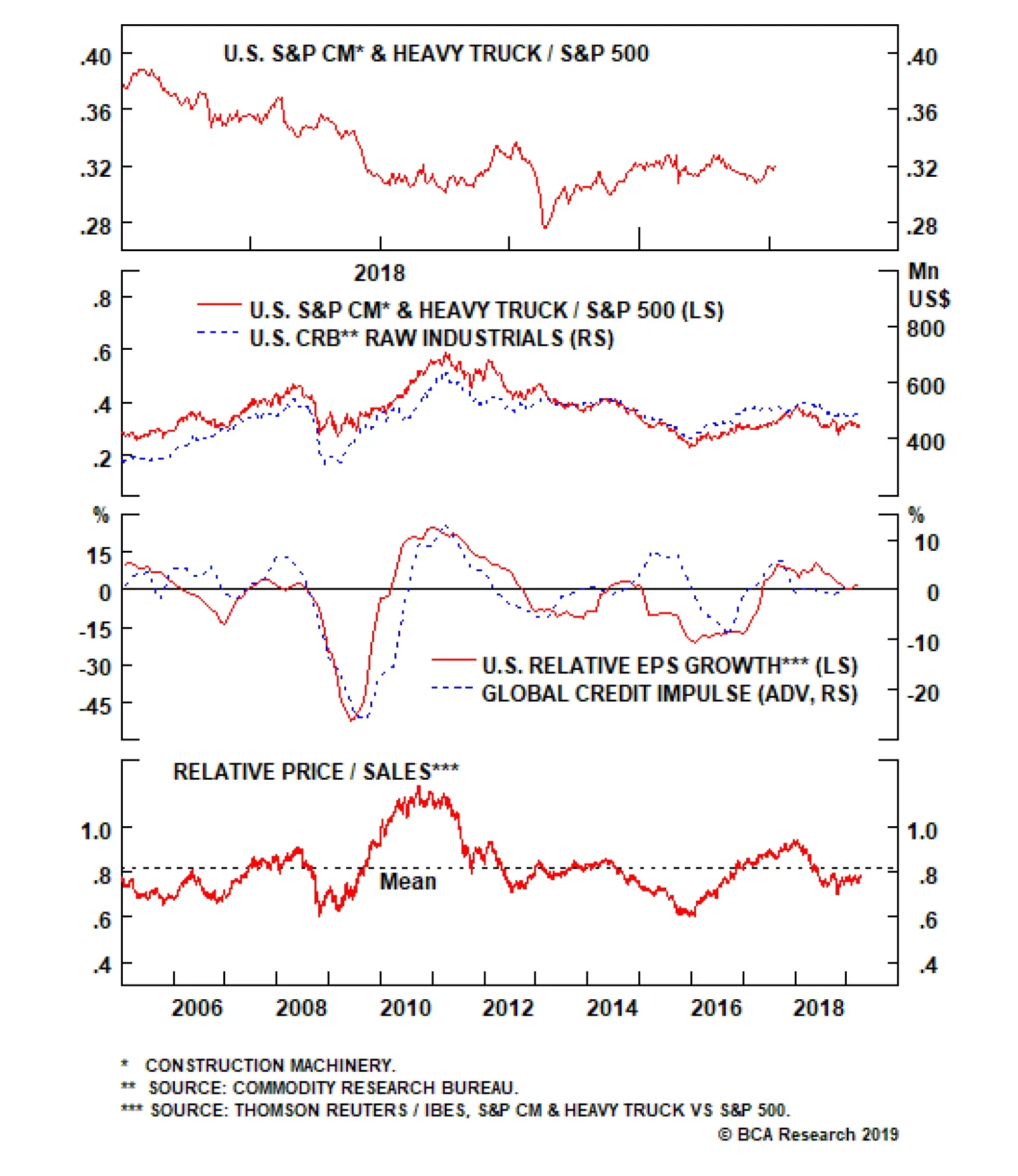
Overweight Caterpillar and, by virtue of its relative dominance, the S&P construction machinery & heavy truck (CMHT) index were at the front of the news cycle this week as an analyst downgraded CAT based on a belief that global growth had collapsed. The market largely ignored the report and both CAT and the S&P CMHT index have continued their outperformance since the late-October trough, when we reiterated our overweight recommendation in our Daily Sector Insight report titled “A Buying Opportunity In Construction Machinery”. The signals from the indicators we track imply that the “global growth collapse” is both late and overstated. The CRB raw industrials index, which moves in lockstep with the S&P CMHT index’s relative performance, unsurprisingly showed weakness at the end of 2018 but has since recovered (second panel). Further, the global credit impulse, an excellent leading indicator of relative profitability, has ticked up into positive territory after sending a weakening signal in 2018 and implies a resumption of profit outperformance (third panel). The combination of positive relative sales growth and still-tepid share price action has taken the relative valuation to levels not seen since the 2015-16 manufacturing recession (bottom panel), which marks an exceptionally affordable entry point, particularly for investors seeking to gain exposure to a China/U.S. trade tussle resolution. We continue to think such buying opportunities are rare and reiterate our overweight recommendation. The ticker symbols for the stocks in this index are: BLBG: S5CSTF - CAT, CMI, PCAR.
Highlights As long as Chinese policymakers remain committed to their anti-pollution campaign, we believe high-grade iron ore prices will remain supported by demand from newer steelmaking technologies. A continuation of the much-needed consolidation in steelmaking capacity in China – wherein larger, more efficient operators force their less competitive rivals from the market – will reinforce this trend (Chart of the Week). Chart of the WeekChina's Steel Sector Will Continue Consolidating
China's Steel Sector Will Continue Consolidating
China's Steel Sector Will Continue Consolidating
Over time, the iron ore market will resemble other developed markets – e.g., crude oil – where higher- and lower-grades of the commodity are regularly traded against each other (Chart 2). As this develops, hedgers and investors will be able to fine tune exposures with greater precision, and prices from these markets will better reflect supply-demand fundamentals. The central and local governments also will have a valuable window on how policy is affecting fundamentals as they pursue their “blue skies” policies. We are initiating tactical spread, getting long spot high-grade 65% Fe vs. short spot 62% Fe at today’s Custeel Seaborne Iron Ore Price Index levels, consistent with our view.1 Chart 2Iron Ore Spread Markets Will Continue To Develop
Iron Ore Spread Markets Will Continue To Develop
Iron Ore Spread Markets Will Continue To Develop
Highlights Energy: Overweight. The Trump administration is reviving the Monroe Doctrine with its demand Russia remove its troops and advisors from Venezuela immediately, based on comments by the U.S. National Security Advisor John Bolton. In addition, a “senior administration official” said waivers for eight of Iran’s largest crude oil importers could be allowed to expire May 4, and that the administration is considering additional sanctions against Iran.2 Brian Hook, the special U.S. envoy for Iran, this week said three of eight countries granted waivers to U.S. sanctions agreed to take oil imports to zero.3 In a related development, OPEC crude oil output fell to a four-year low of 30.4mm b/d in March, according to a Reuters’s survey, as Venezuelan output falls and Saudi Arabia continues to over-deliver on its production cuts. Base Metals: Neutral. Codelco’s mined copper ore output fell to 1.8mm MT last year, down 1.6% vs. 2017 levels. This took refined output down almost 3% to 1.7mm MT, according to Metal Bulletin. The Chilean state-owned company cited reduced ore content in its mined production as a reason for the decline. MB’s copper treatment and refining charges index for the Asia Pacific region is at its lowest level since March 26, 2018, reflecting the lower concentrate supplies. We remain long spot copper on the back of low inventories, and an expected recovery in demand. Precious Metals: Neutral. Strength in equities has taken some of the luster off gold’s rally in the near term as investors move to increase stock exposures, but we continue to favor gold as a portfolio hedge and remain long. Agriculture: Underweight. USDA’s corn planting intentions report released last week came in much stronger than earlier estimates. Corn and soybeans traded lower following the release of the report, but recovered some this week on the back of positive news from Sino - U.S. trade talks. The USDA estimated farmers intended to plant 92mm acres of corn, and 85mm acres of soybeans this year. Ahead of the report, a Farm Bureau survey estimated corn and soybean acreage would average 91.3mm acres of corn and 86.2mm acres of beans. Trade Recommendations: Our 1Q19 trade recommendations were up an average of 41% at end-March (Quarterly Performance Table below). Including recommendations that were open at the beginning of 1Q19, the average was 31%. Feature China’s push to reduce pollution in its steelmaking sector will continue to support demand for Brazil’s high-grade ores – i.e., ores with iron (Fe) content higher than 65%. Transitory Brazilian iron ore supply losses notwithstanding, China’s push to reduce pollution in its steelmaking sector will continue to support demand for Brazil’s high-grade ores – i.e., ores with iron (Fe) content higher than 65%. This will allow the continued development of an active spread market, not unlike spread markets in commodities like oil, which will expand hedging and trading opportunities for producers, consumers and investors (Chart 2). Older, more polluting steelmaking technology in China will continue to be replaced by plants that favor Brazil’s high-grade ores, then Australia’s benchmark-type grades (62% Fe), then, as a last resort, the lower quality domestic ores. In a steelmaking market still suffering significant overcapacity, we expect policymakers will, at some point, discover the benefit of letting markets forces do the work of forcing older technology offline, as happened with the country’s domestically produced lower-quality iron ore, which has lower iron content and higher impurities than Brazilian and Aussie imports.4 We believe growth in China’s steel and steel products demand – hence iron ore demand – likely has peaked and is in the process of flattening or declining slightly, which will alter the composition of iron ore imports and tilt them in favor of high-grade Fe imports from Brazil over the next 3 - 5 years (Chart 3). This leveling off in steel demand growth will put a premium on more efficient technology to meet future demand, particularly with the pollution constraints that will, we believe, be an enduring feature of this market.5 Chart 3China's Steel Demand Growth Likely Has Peaked
China's Steel Demand Growth Likely Has Peaked
China's Steel Demand Growth Likely Has Peaked
Impurities found in lower-grade iron ore raise steelmaking costs by increasing unwanted mineral build-ups in blast furnaces, increase pollution and lower mills’ efficiency. With inventories re-building following the winter steelmaking hiatus in China, imports will continue to grow market share at the expense of indigenous lower-quality ores (Chart 4). Imports from Australia, which mostly price to the 62% Fe benchmark, will continue to grow, but we strongly believe that in China’s post-anti-pollution-campaign market, Brazilian imports will see growth increasing (i.e., the 2nd derivative) at a higher rate (Chart 5). Chart 4Chinese Iron Ore Inventories Fall Relative To Steel Production
Chinese Iron Ore Inventories Fall Relative To Steel Production
Chinese Iron Ore Inventories Fall Relative To Steel Production
Chart 5China's Brazil, Australia Import Growth Will Recover
China's Brazil, Australia Import Growth Will Recover
China's Brazil, Australia Import Growth Will Recover
These imports are lower in cost, and higher in quality than the domestic iron ore. This is particularly important when it comes to keeping costs under control – impurities found in lower-grade iron ore raise steelmaking costs by increasing unwanted mineral build-ups in blast furnaces, increase pollution and lower mills’ efficiency. Extended Output Cuts Favor High-Grade Ores The biggest reason supporting our view high-grade iron ores will continue to grow market share at the expense of lower-quality domestic supply and benchmark 62% Fe material is the recent behavior of the central government and local governments vis-a-vis pollution. Both have shown they are not averse to extending operating restrictions on high-polluting industrial plants, even in provinces where steelmaking is a large employer. Last year, major steel producing regions– Hebei, Jiangsu, Shandong, Liaoning – increased production during the winter months, likely driven by higher margins at the steelmakers (Chart 6). This indicates compliance with anti-pollution regulations fell significantly (Chart 7). In turn, this led to higher pollution, according to the latest available data from China’s National Environmental Monitoring Centre, which shows concentrations of particulate matter 2.5 micrometers or less in diameter (i.e., PM2.5) rose again this year (Chart 8). Chart 6Higher Margins, Higher Output
Higher Margins, Higher Output
Higher Margins, Higher Output
Chart 7
Consequently, Chinese authorities decided to tighten anti-pollution measures by extending production cuts beyond the heating season into 3Q and 4Q19.6 Furthermore, the top producing city, Tangshan, in the province of Hebei extended its most elevated level of smog alert on March 1 and deepened production cuts to 70% from 40%, with reported cases of complete operations being halted. Chart 8China's Pollution Is Increasing; Steelmaking Curbs Will Persist
China's Pollution Is Increasing; Steelmaking Curbs Will Persist
China's Pollution Is Increasing; Steelmaking Curbs Will Persist
Last month, Chinese Communist Party (CCP) officials in Hebei announced plans to cut steel production by 14mm MT this year and next. Going forward, China’s environment ministry said winter restrictions will be extended for a third year during the 2019-2020 winter period. As we argued last year, winter curbs likely will become a permanent feature of China’s steelmaking landscape. Combined with China’s steel de-capacity reforms, iron ore and steel markets will continue to evolve to a less-polluting presence in the country.7 As a consequence, IO grade and form differentials are now crucial input in our analysis.8 We believe a wider than usual premium will remain until new high-grades and pellets supplies come on line in the next few years. Credit Stimulus Vs. Battle For Blue Skies The reversal in China’s credit cycle and in the Fed’s monetary policy stance will be supportive of steel and iron ore prices going forward. In fact, our credit cycle proxy suggests global industrial activity will increase in the next few months (Chart 9).9 Additionally, our geopolitical strategists’ base case suggests a resolution of the Sino-U.S. trade war likely will occur this year. This will support EM income growth, which will stimulate commodity demand generally at the margin. Chart 9Upturn in China's Credit Cycle Will Support Iron Ore Prices
Upturn in China's Credit Cycle Will Support Iron Ore Prices
Upturn in China's Credit Cycle Will Support Iron Ore Prices
We believe China’s credit cycle bottomed in 1Q19 and that Chinese authorities will modestly increase stimulus in 2H19.10 As discussed previously, we do not expect this new round of stimulus to be as large as previous rounds; China’s economy is in better shape now than it was at the start of previous expansionary credit cycles, hence the magnitude of the stimulus needed to revive the economy is lower. Nonetheless, this stimulus will be sufficient to strengthen China’s and EM’s steel-intensive activities in the coming months. As long as China maintains its anti-pollution drive, high-grade iron ore will continue to grow market share. Historically, these sectors correlated positively with the 62% Fe content benchmark (Chart 10). However, the expected stimulus works against Beijing’s critically important battle for blue skies. A revival of China’s industrial activity would increase PM2.5 concentrations above targets. Chart 10China's Stimulus Will Stoke Iron Ore Demand
China's Stimulus Will Stoke Iron Ore Demand
China's Stimulus Will Stoke Iron Ore Demand
These constraints, we believe, mean China’s policymakers will have to incentivize steelmakers to favor lower-polluting high-grade iron ore (Fe > 65%), in order to maximize steel output subject to their emissions target. This will widen the form and grade premiums ahead of next year’s winter period. Bottom Line: As long as China maintains its anti-pollution drive, high-grade iron ore will continue to grow market share, as steelmakers upgrade their technology and inefficient mills are shuttered. This will favor Brazilian exports going forward, and we expect the rate of growth in these imports to increase. In line with our view, we are opening a long 65% Fe spot vs. a short 62% Fe spot position at tonight’s close. This is a tactical position, but could easily become a strategic recommendation. Robert P. Ryan, Senior Vice President Commodity & Energy Strategy rryan@bcaresearch.com Hugo Bélanger, Senior Analyst Commodity & Energy Strategy HugoB@bcaresearch.com Footnotes 1 This index is published by Beijing Custeel E-Commerce Co., Ltd. 2 We flagged this risk in our February 21, 2019, report entitled “The New Political Economy of Oil.” We noted the odds of a U.S. – Russia military confrontation are low, and that “the U.S. would revive the Roosevelt Corollary to the Monroe Doctrine, and that Russia and China most likely would concede Venezuela is within the U.S.’s sphere of influence, as neither intends to project the force and maintain the supply lines … a confrontation would require.” That said, there is always the risk such a confrontation could go kinetic, or that either or both sides could lunch a cyberattack to disable its adversary. The Roosevelt Corollary refers to U.S. President Theodore Roosevelt’s extension of the Monroe Doctrine at the beginning of the 20th century, which has been used by the U.S. to justify the use of military power in the Western Hemisphere. Our February 21 report is available at ces.bcaresearch.com, as is a Special Report on Venezuela published November 22, 2018, entitled “Venezuela: What Cannot Go On Forever Will Stop,” which discusses Venezuela’s debts to China and Russia, et al. See also “Exclusive: Trump eyeing stepped-up Venezuela sanctions for foreign companies – Bolton” and “Oil hits 2019 high on OPEC cuts, concerns over demand ease,” published by reuters.com March 29 and April 2, 2019, respectively. 3 Please see “Three importers cut Iran oil shipments to zero - U.S. envoy” published April 2, 2019, by reuters.com. 4 According to Platts, “at least half of China’s previous 300 million mt plus iron ore mining capacity has left the market for good.” Please see “China’s quest for cleaner skies drives change in iron ore market,” published January 30, 2019, by S&P Global Platts. CRU estimates average iron content in China’s ores is 30%, which means they must undergo costly upgrading to be useful to steelmakers. 5 Australian miners are expected to bring on significant volumes of high-grade iron ore beginning in 2022 - 23, with Fe content as high as 70%, according to the Department of Industry, Innovation and Science’s March 2019 Resources and Energy Quarterly. 6 Please see “Tangshan mulls output curbs for 2nd, 3rd quarters of 2019” published January 22, 2019, by metal.com. 7 Please see China to extend winter anti-smog measures for another year published March 6, 2019, by reuters.com. 8 Grade premium: The chemistry of iron ore supply varies widely in terms of Fe content. Higher Fe content reduces production cost and pollution per unit of steel output. The higher the quality, the higher the volume of steel produced relative to energy consumed. The current global benchmark iron ore is 62% Fe, but China’s evolution to a less-polluting steelmaking sector will raise the importance of higher-grade markets. Form premium: A steelmaker’s blast furnace typically consumes iron ore in pellets, fines or lumps combined with coking coal. Fines are the most common form of iron ore, and account for ~ 75% of total seaborn IO market. This form cannot be directly fed in the blast furnace and requires an extra sintering step. Sintering is highly polluting and coal-intensive process that compresses fines into a more useable form. This process is usually conducted on-site at steel mills. On the other hand, lumps and pellets are direct feedstock and therefore completely avoid the highly polluting sintering step. Both types of premium are primarily affected by environmental policies in consuming countries, coke prices and steelmills’ profitability. 9 Modeling historical iron ore prices remains difficult because of the short sample available for spot iron prices – i.e., the benchmark 62% Fe. Before 2009, iron ore prices were determined using a producer pricing system. Once a year, prices were negotiated by miners and steelmakers and would be fixed for the remaining of the year. Given that iron ore supply was plentiful relative to demand, prices were fairly stable and this mechanism was used for over four decades. The rapid rise of emerging economies – mainly China – during the 2000s forced the pricing system to adjust toward a spot-market pricing system. The short spot-price time series available for analysis increases the distortion of policy-driven exogenous shocks like China’s de-capacity and winter restriction policies. This makes it difficult to identify the underlying relationships between its price and potential explanatory variables, and forces us to rely on theory and analogous experience in other markets like crude oil. 10 Please see BCA Commodity and Energy Strategy Weekly Report titled “Bottoming Of China’s Credit Cycle Bullish For Copper Over Near Term,” published March 14, 2019. It is available at ces.bcaresearch.com Investment Views and Themes Recommendations Strategic Recommendations Tactical Trades Trade Recommendation Performance In 2019 Q1
Image
Commodity Prices and Plays Reference Table Trades Closed in 2019 Summary of Closed Trades
Image
Conglomerates Have Been Rerating
Conglomerates Have Been Rerating
Overweight (Downgrade Alert) Last fall we felt all of the shoes had dropped in the S&P industrial conglomerates index: industrial conglomerate stalwart GE had cut their dividend to a token to $0.01 per share following awful guidance and the other key constituent members, MMM and HON, noted tariffs and trade wars factoring heavily in their own respective guidance cuts. The market had moved to a deeply negative position with valuations at post-GFC lows which we took as a contrarily positive signal that sentiment had moved too far and we upgraded the index to overweight based on valuations. Our call was somewhat early; GE took another month to reach a 20-yr low. However, since then the index has been smartly outperforming the broad market as GE has surged nearly 50% from the bottom and our expectation of a rerating has largely panned out (second and bottom panels). Bottom Line: With a valuation rerating underway, our contrarian thesis is weakening and we are compelled to add a downgrade alert. We believe this heavily international index would be a key beneficiary of easing in the U.S./China trade tussle which we anticipate to be the catalyst to execute our downgrade alert. The ticker symbols for the stocks in this index are: BLBG: S5INDCX - GE, MMM, HON, ROP.
A Rare Opportunity In Defense Stocks
A Rare Opportunity In Defense Stocks
Overweight Though the pure-play BCA defense index has retreated somewhat from the mid-2018 highs, our thesis remains solidly on the offensive. As a reminder, we have been overweight the pure-play BCA defense index since late-2015 and our strategy has been to add exposure on any meaningful pullbacks and keep this index as a structural overweight within the GICS1 S&P industrials index; we believe the current environment is an excellent opportunity to increase exposure. The timing of the current pullback is curious as it has occurred simultaneous to the rapid increase in defense outlays (second panel). Importantly, the CBO projects this level of spending to persist, even without a wartime buildup, as the upgrade of the military remains a core Trump administration policy goal. Considering the relative price of defense stocks is at roughly the same level as it was immediately before the 2016 election (top panel), little of this largesse appears to be priced in. The key offset to our bullish thesis was that valuations in the defense sector were high. However, that negative has evaporated along with the sector’s premium valuation since the beginning of 2019 (bottom panel). Accordingly, we reiterate our overweight recommendation. The ticker symbols for the stocks in the BCA defense index are: LMT, LLL, NOC, GD and RTN.
Highlights Chart 1What’s The Downside?
What’s The Downside?
What’s The Downside?
How low can it go? This is the question most investors are asking these days about the 10-year Treasury yield. Our answer is that it can’t go much lower unless the U.S. economy falls into recession, an event we don’t anticipate in 2019. Considering the main macro drivers of the 10-year Treasury yield, we find that the Global Manufacturing PMI (Chart 1), U.S. dollar bullish sentiment (not shown) and Global Economic Policy Uncertainty (not shown) are all close to mid-2016 levels. In other words, the economic growth and policy environment is almost identical to the one that produced a 1.37% 10-year Treasury yield in mid-2016. What’s preventing a return to mid-2016 yield levels is that the Fed has delivered nine rate hikes since then, and rising wage growth confirms that the output gap has closed considerably (bottom panel). In other words, with short-maturity yields much higher than three years ago, we would need to see a much more pronounced growth slowdown, i.e. PMIs well below 50, to re-produce a sub-2% 10-year Treasury yield. If 2019 continues to follow the 2016 roadmap and the Global PMI bottoms-out around 50, then the 10-year Treasury yield has probably already found its floor. Feature Investment Grade: Overweight Investment grade corporate bonds outperformed the duration-equivalent Treasury index by 24 basis points in March, bringing year-to-date excess returns up to +268 bps. The Federal Reserve’s pause opens a window for corporate spreads to tighten during the next few months. We recommend overweight positions in corporate bonds for now, but will be quick to reduce exposure once spreads reach our near-term targets. Aaa spreads are already below target levels and we recommend avoiding that credit tier. Other credit tiers still have room to tighten, though Aa and A-rated bonds are only 3 bps and 5 bps above target, respectively (Chart 2).1 Once spreads reach more reasonable levels for this phase of the cycle, we will be quick to reduce corporate bond exposure because some indicators of corporate default risk are already sending warning signals.2 Most notably, corporate profits grew only 4.0% (annualized) in Q4 2018 while corporate debt rose 5.3% (annualized). The result is that our measure of gross leverage ticked higher for the first time since Q3 2017 (bottom panel). Going forward, with corporate profit growth likely to stabilize in the mid-single digit range, gross leverage will probably stay close to its current level. That would be consistent with a 3% speculative grade default rate, significantly above the 1.7% rate currently projected by Moody’s. Chart 2Investment Grade Market Overview
Investment Grade Market Overview
Investment Grade Market Overview
Chart
Chart
High-Yield: Overweight High-Yield underperformed the duration-equivalent Treasury index by 23 basis points in March, dragging year-to-date excess returns down to +566 bps. Junk spreads for all credit tiers remain above our near-term spread targets.3 At present, the Ba-rated option-adjusted spread is 235 bps, 55 bps above our target. The B-rated spread is 285 bps, 102 bps above our target. The Caa-rated spread is 802 bps, 244 bps above our target (Chart 3). Chart 3High-Yield Market Overview
High-Yield Market Overview
High-Yield Market Overview
Elevated spreads mean that investors are currently well compensated for default risk, but that could change later in the year. In a recent report we showed that some leading default indicators – gross leverage, C&I lending standards and job cut announcements (bottom panel) – are showing signs of deterioration.4 Specifically, our model suggests that the speculative grade default rate could be 3% or higher during the next 12 months. Moody’s currently forecasts 1.7%. If the Moody’s forecast is correct, the high-yield default adjusted spread is 306 bps. If the Moody’s forecast turns out to be correct, then investors will take home a default-adjusted spread of 306 bps, well above the historical average of 250 bps. If our 3% forecast is correct, then the default-adjusted spread falls to 230 bps, slightly below the historical average (panel 4). In either case, investors are reasonably well compensated for bearing default risk, but that will change when spreads reach our near-term targets. We will be quick to cut exposure at that time. MBS: Neutral Mortgage-Backed Securities underperformed the duration-equivalent Treasury index by 11 basis points in March, dragging year-to-date excess returns down to +27 bps. The conventional 30-year zero-volatility spread widened 3 bps on the month, driven entirely by an increase in the compensation for prepayment risk (option cost). The option-adjusted spread (OAS) held flat at 40 bps. Falling mortgage rates since the beginning of the year have caused an increase in refinancing activity, leading to some widening in nominal MBS spreads (Chart 4). However, the tepid pace of new issuance in recent years means that the existing mortgage stock is not very exposed to refinancing risk. Consider that, despite an 80 bps drop in the 30-year mortgage rate, the MBA Refinance index has only risen to 1290. The Refi index’s historical average is 1824. Chart 4MBS Market Overview
MBS Market Overview
MBS Market Overview
Further, housing starts and new home sales appear to have stabilized, meaning that there is probably not much further downside for mortgage rates. As a consequence, we don’t see much more scope for MBS spread widening. While MBS spreads appear relatively safe, the sector does not offer attractive expected returns compared to the investment alternatives. For example, the index option-adjusted spread for conventional 30-year MBS is well below its average historical level (panel 3) and the sector offers less compensation than normal compared to corporate bonds (panel 4). MBS also offer a poor risk/reward trade-off compared to other Aaa-rated spread products, as we showed in a recent report.5 Government-Related: Underweight The Government-Related index outperformed the duration-equivalent Treasury index by 23 basis points in March, bringing year-to-date excess returns up to +115 bps. Sovereign debt outperformed duration-equivalent Treasuries by 13 bps on the month, bringing year-to-date excess returns up to +334 bps. Local Authorities outperformed the Treasury benchmark by 53 bps and Foreign Agencies outperformed by 42 bps, bringing year-to-date excess returns up to +139 bps and +151 bps, respectively. Domestic Agencies outperformed by 11 bps in March, bringing year-to-date excess returns up to +20 bps. Supranationals outperformed by 4 bps, bringing year-to-date excess returns up to +16 bps. The USD-denominated sovereign debt of most countries continues to look expensive relative to equivalently-rated U.S. corporate credit. However, in a recent report we highlighted that Mexican sovereign debt is an exception (Chart 5).6 Chart 5Government-Related Market Overview
Government-Related Market Overview
Government-Related Market Overview
Not only is Mexican sovereign debt cheap relative to U.S. corporates, but our Emerging Markets Strategy service has shown that the Mexican peso is cheap.7 The prospect of a stronger peso versus the U.S. dollar makes the spread on offer from Mexican sovereign debt look even more attractive. Municipal Bonds: Overweight Municipal bonds underperformed the duration-equivalent Treasury index by 39 basis points in March, dragging year-to-date excess returns down to +52 bps (before adjusting for the tax advantage). The average Aaa-rated Municipal / Treasury yield ratio rose 1% in March, and currently sits at 82% (Chart 6). This is more than one standard deviation below its post-crisis mean and right around the average of 81% that prevailed in the late stages of the previous cycle, between mid-2006 and mid-2007. Chart 6Municipal Market Overview
Municipal Market Overview
Municipal Market Overview
The Municipal / Treasury yield ratio for short maturities (2-year and 5-year) remains well below the yield ratio for longer maturities (10-year, 20-year and 30-year). In other words, the best value in the municipal bond space is at the long-end of the curve, and we continue to recommend that investors favor those maturities. Recently released data from the Bureau of Economic Analysis shows that state & local government revenue growth declined in Q4 2018, for the first time since Q2 2017. As a result, our measure of state & local government interest coverage fell from a lofty 17 all the way down to 5 (bottom panel). Positive interest coverage means that state & local governments are still generating sufficient revenue to cover current expenditures and interest payments, and we therefore don’t anticipate a surge in muni ratings downgrades any time soon. We also continue to note that municipal bonds tend to perform better in the middle-to-late phases of the economic cycle, while corporate credit delivers its best returns early in the recovery.8 Investors should maintain an overweight allocation to municipal debt. Treasury Curve: Adopt A Barbell Curve Positioning Treasury yields fell dramatically in March, as the Fed surprised markets with a larger-than-expected downward revision to its interest rate projections. The result is that the overnight index swap curve is now priced for 34 basis points of rate cuts over the next 12 months (Chart 7). Chart 7Treasury Yield Curve Overview
Treasury Yield Curve Overview
Treasury Yield Curve Overview
The 2/10 Treasury slope flattened 7 bps to end the month at 14 bps. The 5/30 slope steepened 1 bp to end the month at 58 bps. In recent reports we urged investors to adopt barbell positions along the yield curve. In particular, investors should avoid the 5-year and 7-year maturities and instead focus their allocations at the very short and long ends of the curve.9 There are three main reasons to prefer a barbell positioning. First, the 5-year and 7-year yields are most sensitive to changes in our 12-month discounter. In other words, those yields fall the most when the market prices in rate cuts and rise the most when it prices in rate hikes. As long as recession is avoided, the market will eventually price rate hikes back into the curve. Favor the 2/30 barbell over the 7-year bullet. Second, barbells currently offer a yield pick-up relative to bullets. The duration-matched 2/10 barbell offers 10 bps more yield than the 5-year bullet (panel 4), and the duration-matched 2/30 barbell offers 9 bps more yield than the 7-year bullet. This means that investors will earn positive carry in barbell positions while they wait for rate hikes to get priced back in. Finally, all barbell combinations look cheap according to our yield curve fair value models (see Appendix B). TIPS: Overweight TIPS underperformed the duration-equivalent nominal Treasury index by 44 basis points in March, dragging year-to-date excess returns down to +76 bps. The 10-year TIPS breakeven inflation rate fell 7 bps to end the month at 1.88% (Chart 8). The 5-year/5-year forward TIPS breakeven inflation rate fell 8 bps to end the month at 1.98%. Both rates remain below the 2.3% - 2.5% range that has historically been consistent with inflation expectations that are well-anchored around the Fed’s target. Chart 8Inflation Compensation
Inflation Compensation
Inflation Compensation
As we noted in last week’s report, with financial conditions no longer excessively easy, the Fed has pivoted to a more dovish stance in an effort to re-anchor inflation expectations at levels more consistent with its 2% target.10 This change should support wider TIPS breakevens, though investors will also need to see evidence of firming realized inflation before meaningful upside materializes. So far, such evidence is in short supply. Note that trimmed mean PCE inflation has rolled over again after having just touched 2% (bottom panel). Trimmed mean PCE is running at 1.84% year-over-year. Nevertheless, we would maintain an overweight allocation to TIPS versus nominal Treasuries. First, our commodity strategists see further upside in the price of oil (panel 2), and second, the 10-year TIPS breakeven inflation rate is 6 bps too low relative to the fair value from our Adaptive Expectations model (panel 4).11 ABS: Underweight Asset-Backed Securities outperformed the duration-equivalent Treasury index by 2 basis points in March, bringing year-to-date excess returns up to +40 bps. The index option-adjusted spread for Aaa-rated ABS widened 2 bps on the month and currently sits at 34 bps, exactly equal to its pre-crisis low (Chart 9). Chart 9ABS Market Overview
ABS Market Overview
ABS Market Overview
We showed in a recent report that Aaa-rated consumer ABS offer a relatively poor risk/reward trade-off compared to other U.S. fixed income sectors, a result that is echoed by the Excess Return Bond Map in Appendix C.12 This should not be surprising given that Aaa ABS spreads are close to all-time lows. What is surprising is that ABS spreads are so tight while the consumer delinquency rate is rising (panel 3). Although the delinquency rate remains well below pre-crisis levels, it will likely continue to rise going forward. Household interest payments are rising quickly as a share of disposable income (panel 3) and banks are tightening lending standards for both credit cards and auto loans (bottom panel). We recommend an underweight allocation to consumer ABS, preferring to take Aaa spread risk in MBS and CMBS. Non-Agency CMBS: Neutral Non-Agency Commercial Mortgage-Backed Securities outperformed the duration-equivalent Treasury index by 5 basis points in March, bringing year-to-date excess returns up to +146 bps. The index option-adjusted spread for non-agency Aaa-rated CMBS widened 2 bps to end the month at 73 bps, below its average pre-crisis level but somewhat higher than recent tights (Chart 10). Chart 10CMBS Market Overview
CMBS Market Overview
CMBS Market Overview
In a recent report we noted that non-agency CMBS offer the best risk/reward trade-off of any Aaa-rated U.S. spread product.13 While we remain cautious on the macro outlook for commercial real estate, noting that prices are decelerating (panel 3) and banks are tightening lending standards (panel 4) amidst falling demand (bottom panel), we view elevated CMBS spreads as providing reasonable compensation for this risk for the time being. Agency CMBS: Overweight Agency CMBS underperformed the duration-equivalent Treasury index by 2 basis points in March, dragging year-to-date excess returns down to +74 bps. The index option-adjusted spread widened 2 bps on the month and currently sits at 50 bps. The Excess Return Bond Map in Appendix C shows that Agency CMBS offer high potential return compared to other low-risk spread products. An overweight allocation to this defensive sector remains appropriate. Appendix A - The Golden Rule Of Bond Investing We follow a two-step process to formulate recommendations for bond portfolio duration. First, we determine the change in the federal funds rate that is priced into the yield curve for the next 12 months. Second, we decide – based on our assessments of the economy and Fed policy – whether the change in the fed funds rate will exceed or fall short of what is priced into the curve. Most of the time, a correct answer to this question leads to the appropriate duration call. We call this framework the Golden Rule Of Bond Investing, and we demonstrated its effectiveness in the U.S. Bond Strategy Special Report, “The Golden Rule Of Bond Investing”, dated July 24, 2018, available at usbs.bcaresearch.com. Chart 11 illustrates the Golden Rule’s track record by showing that the Bloomberg Barclays Treasury Master Index tends to outperform cash when rate hikes fall short of 12-month expectations, and vice-versa. At present, the market is priced for 34 basis points of cuts during the next 12 months. We do not anticipate any rate cuts during this timeframe, and therefore recommend that investors maintain below-benchmark portfolio duration. Chart 11The Golden Rule's Track Record
The Golden Rule's Track Record
The Golden Rule's Track Record
We can also use our Golden Rule framework to make 12-month total return and excess return forecasts for the Bloomberg Barclays Treasury index under different scenarios for the fed funds rate. Excess returns are relative to the Bloomberg Barclays Cash index. To forecast total returns we first calculate the 12-month fed funds rate surprise in each scenario by comparing the assumed change in the fed funds rate to the current value of our 12-month discounter. This rate hike surprise is then mapped to an expected change in the Treasury index yield using a regression based on the historical relationship between those two variables. Finally, we apply the expected change in index yield to the current characteristics (yield, duration and convexity) of the Treasury index to estimate total returns on a 12-month horizon. The below tables present those results, along with 95% confidence intervals. Excess returns are calculated by subtracting assumed cash returns in each scenario from our total return projections.
Image
Image
Appendix B - Butterfly Strategy Valuation The following tables present the current read-outs from our butterfly spread models. We use these models to identify opportunities to take duration-neutral positions across the Treasury curve. The following two Special Reports explain the models in more detail: U.S. Bond Strategy Special Report, “Bullets, Barbells And Butterflies”, dated July 25, 2017, available at usbs.bcaresearch.com U.S. Bond Strategy Special Report, “More Bullets, Barbells And Butterflies”, dated May 15, 2018, available at usbs.bcaresearch.com Table 4 shows the raw residuals from each model. A positive value indicates that the bullet is cheap relative to the duration-matched barbell. A negative value indicates that the barbell is cheap relative to the bullet. Table 5 scales the raw residuals in Table 4 by their historical means and standard deviations. This facilitates comparison between the different butterfly spreads. Table 6 flips the models on their heads. It shows the change in the slope between the two barbell maturities that must be realized during the next six months to make returns between the bullet and barbell equal. For example, a reading of +53 bps in the 5 over 2/10 cell means that we would only expect the 5-year to outperform the 2/10 if the 2/10 slope steepens by more than 53 bps during the next six months. Otherwise, we would expect the 2/10 barbell to outperform the 5-year bullet. Table 4Butterfly Strategy Valuation: Raw Residuals In Basis Points (As of March 29, 2019)
Finding The Floor
Finding The Floor
Table 5Butterfly Strategy Valuation: Standardized Residuals (As of March 29, 2019)
Finding The Floor
Finding The Floor
Table 6Discounted Slope Change During Next 6 Months (BPs)
Finding The Floor
Finding The Floor
Appendix C - Excess Return Bond Map The Excess Return Bond Map is used to assess the relative risk/reward trade-off between different sectors of the U.S. fixed income market. The Map employs volatility-adjusted breakeven spread analysis to show how likely it is that a given sector will earn/lose money during the subsequent 12 months. The Map does not incorporate any macroeconomic view. The horizontal axis of the Map shows the number of days of average spread widening required for each sector to lose 100 bps versus a position in duration-matched Treasuries. Sectors plotting further to the left require more days of average spread widening and are therefore less likely to see losses. The vertical axis shows the number of days of average spread tightening required for each sector to earn 100 bps in excess of duration-matched Treasuries. Sectors plotting further toward the top require fewer days of spread tightening and are therefore more likely to earn 100 bps of excess return.
Chart 12
Ryan Swift, U.S. Bond Strategist rswift@bcaresearch.com Jeremie Peloso, Research Analyst jeremiep@bcaresearch.com Footnotes 1 For further details on how we arrive at those spread targets please see U.S. Bond Strategy Weekly Report, “Paid To Wait”, dated February 26, 2019, available at usbs.bcaresearch.com 2 Please see U.S. Bond Strategy Special Report, “Assessing Corporate Default Risk”, dated March 19, 2019, available at usbs.bcaresearch.com 3 For further details on how we arrive at our spread targets please see U.S. Bond Strategy Weekly Report, “Paid To Wait”, dated February 26, 2019, available at usbs.bcaresearch.com 4 Please see U.S. Bond Strategy Special Report, “Assessing Corporate Default Risk”, dated March 19, 2019, available at usbs.bcaresearch.com 5 Please see U.S. Bond Strategy Weekly Report, “The Search For Aaa Spread”, dated March 12, 2019, available at usbs.bcaresearch.com 6 Please see U.S. Bond Strategy Weekly Report, “The Value In Corporate Bonds”, dated February 19, 2019, available at usbs.bcaresearch.com 7 Please see Emerging Markets Strategy Weekly Report, “Dissecting China’s Stimulus”, dated January 17, 2019, available at ems.bcaresearch.com 8 Please see U.S. Bond Strategy Special Report, “2019 Key Views: Implications For U.S. Fixed Income”, dated December 11, 2018, available at usbs.bcaresearch.com 9 Please see U.S. Bond Strategy Weekly Report, “Paid To Wait”, dated February 26, 2019, available at usbs.bcaresearch.com 10 Please see U.S. Bond Strategy Weekly Report, “The New Battleground For Monetary Policy”, dated March 26, 2019, available at usbs.bcaresearch.com 11 For further details on the model please see U.S. Bond Strategy Weekly Report, “Adaptive Expectations In The TIPS Market”, dated November 20, 2018, available at usbs.bcaresearch.com 12 Please see U.S. Bond Strategy Weekly Report, “The Search For Aaa Spread”, dated March 12, 2019, available at usbs.bcaresearch.com 13 Please see U.S. Bond Strategy Weekly Report, “The Search For Aaa Spread”, dated March 12, 2019, available at usbs.bcaresearch.com Fixed Income Sector Performance Recommended Portfolio Specification Corporate Sector Relative Valuation And Recommended Allocation
Feature GAA DM Equity Country Allocation Model Update The GAA DM Equity Country Allocation model is updated as of March 29, 2019. The quant model has not made changes in the direction of underweights and overweights compared to last month. However, the magnitude of the U.S underweight was reduced, so was that of the overweights in Spain and Germany, as shown in Table 1. Table 1Model Allocation Vs. Benchmark Weights
GAA Quant Model Updates
GAA Quant Model Updates
As shown in Table 2 and Charts 1 - 3, the overall model underperformed the MSCI world benchmark by 44 bps in March, with a 45 bps of underperformance from the Level 2 model and a 20 bps of underperformance from Level 1. What has contributed to such an underperformance? As shown in Chart 4, directionally, 7 out of the 12 country allocations generated positive alpha, however, the negative value added from the overweights in Germany and Spain overwhelmed all the positives. This shows again that quant models with a “systematic” approach cannot fully capture “atypical” conditions in the market place. This is one of the reasons that we use (and also have suggested our clients to use) our quant models as a starting point in the decision-making process, but to use them together with human judgement. Table 2Performance (Total Returns In USD %)
GAA Quant Model Updates
GAA Quant Model Updates
Chart 1GAA DM Model Vs. MSCI World
GAA DM Model Vs. MSCI World
GAA DM Model Vs. MSCI World
Chart 2GAA U.S. Vs. Non U.S. Model (Level 1)
GAA U.S. Vs. Non U.S. Model (Level 1)
GAA U.S. Vs. Non U.S. Model (Level 1)
Chart 3GAA Non U.S. Model (Level 2)
GAA Non U.S. Model (Level 2)
GAA Non U.S. Model (Level 2)
Chart 4
Please see also the website http://gaa.bcaresearch.com/trades/allocation_performance. For more details on the models, please see Special Report, “Global Equity Allocation: Introducing The Developed Markets Country Allocation Model,” dated January 29, 2016, available at https://gaa.bcaresearch.com. Please note that the overall country and sector recommendations published in our Monthly Portfolio Update and Quarterly Portfolio Outlook use the results of these quantitative models as one input, but do not stick slavishly to them. We believe that models are a useful check, but structural changes and unquantifiable factors need to be considered too in making overall recommendations. GAA Equity Sector Selection Model The GAA Equity Sector Model (Chart 5) is updated as of March 29, 2019. Chart 5Overall Model Performance
Overall Model Performance
Overall Model Performance
Table 3Model’s Performance (March 1, 2019 - Current)
GAA Quant Model Updates
GAA Quant Model Updates
Table 4Current Model Allocations
GAA Quant Model Updates
GAA Quant Model Updates
Following the changes implemented and the model relaunch last month, the model continues to maintain a slightly cyclical stance by overweighting Industrials and Materials. The relative tilts within cyclicals and defensives remains the same as the previous month. Global growth concerns still prevent the model from being outright bullish on cyclicals. The valuation component remains muted across all sectors. The model is still overweight Utilities due to positive inputs from its momentum and liquidity components. For more details on the model, please see the Special Report “Introducing the GAA Equity Sector Selection Model,” dated July 27, 2016, as well as the Sector Selection Model section in the Special Alert “GAA Quant Model Updates,” dated March 1, 2019 available at https://gaa.bcaresearch.com. Xiaoli Tang, Associate Vice President xiaoliT@bcaresearch.com Amr Hanafy, Research Associate amrh@bcaresearch.com
Highlights U.S. growth remains robust, despite some temporary softness in recent months. Ex U.S., growth continues to fall but, with China probably now ramping up monetary stimulus, should bottom in the second half. Central banks everywhere have turned more dovish, partly in an attempt to push up inflation expectations. The combination of resilient growth and easier monetary policy should be good for global equities. We remain overweight equities versus bonds. Bond yields have fallen sharply everywhere. However, with U.S. inflation still trending up, and central banks unlikely to turn any more dovish this year, yields are unlikely to fall much further in 2019. We recommend a slight underweight on duration. We remain overweight U.S. equities, but are on watch to upgrade the euro zone and Emerging Markets when we have stronger conviction about China’s stimulus. Given structural headwinds in both Europe and EM, this would probably be only a tactical upgrade. We have been tilting our equity sector recommendations in a more cyclical direction, last month raising Industrials and Energy to overweight. We also prefer credit over government bonds within the fixed-income category, though we warn that spreads will not fall much further given weak corporate fundamentals. Feature Recommended Allocation
Quarterly - April 2019
Quarterly - April 2019
Overview Don’t Fight The Doves The performance of risk assets essentially comes down to a battle between growth and monetary policy/interest rates. Last September, despite the fact that global economic growth was clearly slowing, the Fed sounded hawkish; this triggered an 18% drop in global equities in Q4. But, since late last year, all major developed central banks have turned more dovish, culminating in March’s decision of the ECB to push back its guidance for its first rate hike, and the FOMC’s wiping out its two planned hikes for 2019. But, at the same time, U.S. economic growth is showing resilience, and we see the first “green shoots” of a cyclical pickup in growth outside the U.S. This is an environment in which risk assets should continue to perform well. Why did the Fed back off? The most likely explanation is that it wants to give itself more room to act come the next recession. Inflation expectations have become unanchored, with 10-year breakevens over the past decade steadily below a level that would be consistent with the Fed achieving its 2% core PCE inflation target in the long run. In the period since the Fed formally introduced this (supposedly “symmetrical”) target in 2012, it has exceeded it in only four months (Chart 1). Around recessions over the past 50 years, the Fed has on average cut rates by 655 basis points (Table 1). It sees little risk, therefore, in letting the economy “run a little hot” and allowing inflation to rise somewhat above 2%. This would reanchor expectations, and eventually get nominal short- and long-term rates higher before the next recession. Chart 1Market Doesn’t Believe The Fed’s Target
Market Doesn't Believe The Fed's Target
Market Doesn't Believe The Fed's Target
Table 1Fed Won’t Be Able To Cut This Much Next Time
Quarterly - April 2019
Quarterly - April 2019
Chart 2Financial Conditions Now Much Easier
Financial Conditions Now Much Easier
Financial Conditions Now Much Easier
Chart 3Housing Market Bottoming Out
Housing Market Bottoming Out
Housing Market Bottoming Out
Meanwhile, U.S. growth seems to be stabilizing at a decent level after signs of weakness late last year caused by tighter financial conditions, a slowdown elsewhere in the world, and the six-week government shutdown. An easing of financial conditions since the beginning of the year should help to keep U.S. GDP growth above trend at around 2.0-2.5% this year (Chart 2). Most notably, interest-rate sensitive areas of the economy that were under pressure last year, especially housing, are showing signs of bottoming (Chart 3). Consumption also should be robust, given strong wage growth, consumer confidence close to historic record high levels, and amid no signs of a deterioration in the labor market (Chart 4). Chart 4No Signs Of Weaker Labor Market
No Signs Of Weaker Labor Market
No Signs Of Weaker Labor Market
Chart 5Some 'Green Shoots' For Global Growth
Some "Green Shoots" For Global Growth
Some "Green Shoots" For Global Growth
A key question for us over the next few months will be when to shift allocations to more cyclical, higher-beta equity markets such as the euro area and Emerging Markets. These have underperformed year-to-date despite the strong risk-on market. China’s nascent reflationary stimulus will decide the timing and level of conviction of this shift. As we explain in detail on page 6, we think the jury is still out on whether China is injecting liquidity on anything like the same scale as it did in 2016. Even if it is, historically it has taken six to 12 months before the effect showed through via a rebound in global trade, commodity prices, and other China-related indicators. The first early signs of a bottoming are emerging: Chinese fixed-asset investment and the Caixin Manufacturing PMI beat expectations last month, the German ZEW Expectations indicator has started to recover, and the diffusion index of the Global Leading Economic Indicator (which often leads the LEI itself by a few months) has picked up (Chart 5). We are on watch to shift our allocation1 but, given the long-term structural headwinds against both Europe and EM, we need to be more convinced about the strength of Chinese stimulus before doing so. The seeds of recession are sown in expansions. Eventually, we see the newly dovish Fed falling behind the curve. The Fed Funds Rate is still below the range of estimates of the neutral rate – hard though this is to estimate in real time (Chart 6). If the economy remains as strong as we expect, sometime next year inflation could begin rising to uncomfortable levels (and asset bubbles start to be of concern), which would push the Fed back into hiking mode. Given that the market is pricing in Fed rate cuts, not hikes, and that the Fed can hardly sound any more dovish than it does now without moving to an outright easing path, it seems to us that long-term rates are very unlikely to fall from here (Chart 7). Chart 6Fed Still Below Neutral
Fed Still Below Neutral
Fed Still Below Neutral
Chart 7Can The Fed Get Any More Dovish Than This?
Can The Fed Get Any More Dovish Than This?
Can The Fed Get Any More Dovish Than This?
In this environment, therefore, we continue to expect global equities to outperform bonds over the next 12 months. However, a recession is possible in 2021 triggered by the Fed late next year needing to put its foot abruptly on the brake. What Our Clients Are Asking Chart 8Ex-U.S. Equities Driven By China Stimulus
Ex US Equities Driven By China Stimilus
Ex US Equities Driven By China Stimilus
When Is The Time To Switch Allocations To Europe And EM? It is slightly surprising that the 12% rally in global equities this year has been led by the low-beta U.S., up 13%, rather than Europe (up 9%) or emerging markets (up 9% - and much less if the strong Chinese market is excluded). Is it time to switch to these underperforming, more cyclical markets? Our answer is, not yet. Global growth ex-U.S. continues to weaken. It is likely to bottom sometime in the second half, as a result of Chinese growth stabilizing. However, the jury is still out on whether the increase in Chinese credit creation in January was a one-off, or major policy reversal. Even if it is the latter, a revival in global growth (and cyclical markets) has typically lagged Chinese stimulus by 6-12 months (Chart 8, panel 1). There are also significant structural headwinds for both the euro zone and Emerging Markets which make us reluctant to overweight them unless there are clear cyclical reasons to do so. Both have lagged global equities fairly consistently since the Global Financial Crisis, with only brief outperformance during periods of economic acceleration, such as in 2016 and 2012 (panel 2). The euro zone remains challenged by its banking system. Loan growth has been stagnant for years, and banks remain undercapitalized relative to their U.S. peers, and highly fragmented (panels 3 and 4). Emerging markets are hampered by their high level of foreign-currency debt (which makes them highly sensitive to U.S. financial conditions), dependence on China, and lack of structural reform. We could see ourselves shifting our recommendation from the U.S. to the euro area and EM, and becoming outright bearish on the U.S. dollar (a counter-cyclical currency), over the coming months if we find confirmation of a bottoming of global cyclical growth and become more confident in the size of China’s stimulus. But given the structural headwinds, and the steady underperformance of these markets, we need stronger evidence first. Chart 9Oil, Positioning, And Housing
Oil, Positioning, And Housing
Oil, Positioning, And Housing
Why Is The 10-Year Bond Yield So Depressed? Despite U.S. equities rallying back to within 4% of a record high, the U.S. Treasury bond yield has fallen further this year (Chart 9, panel 1). Moreover, the 3-month/10-year yield curve has briefly inverted. Besides the Fed’s recent more dovish turn, what has depressed bond yields? We would pin the cause on the following factors: Dampened inflation expectations: Over the past few years the 10-year yield has been closely correlated with the oil price via inflation expectations. A temporary supply shock in Q4 caused oil prices to decline sharply. But tighter supply this year should allow the oil price to recover further. This should cause a rise in inflation expectation (panel 2). Trade positioning: Late last year, speculative short positions in government bonds were at their highest levels since 2015. However, the Q4 equity selloff pushed investors to cover their positions; these are now close to neutral (panel 3). Home Sales: Housing data has been weak over the past few quarters, with both existing and new home sales declining. But there are now signs of recovery: mortgage applications have started to pick up, which should in turn push home sales higher (panel 4). This should also allow for a rise in bond yields. Our key take-away from March’s FOMC meeting, when the tone turned decidedly dovish, is that the Fed is focusing on re-anchoring inflation expectations, which should push nominal yields higher. We think the market is very pessimistic by pricing in 42 and 56 bps of rate cuts over the next 12 and 24 months respectively. It would take a significant further weakening of economic data to make the Fed’s stance turn even more dovish and for nominal yields to fall even further. How Will U.S. Corporate Bonds Perform In The Next Recession? Historically high levels of U.S. corporate debt, as well as declining credit quality in the investment-grade space, have started to worry investors (Chart 10). Specifically, investors are worried that, when the next default cycle comes, a large portion of investment-grade debt will be downgraded to junk, forcing fund managers who are constrained to hold certain credit qualities to sell. These worries seem to be justified. Investment-grade bonds of lower credit quality tend to experience large increases in migration to junk status during credit recessions (Chart 11). Given the current composition of the U.S. investment-grade corporate bond universe, a credit recession would imply a downgrade to junk status of 4.6% of the index if we assume similar behavior to previous recessions. Depending on the speed of the selloff, such a downgrade could also have grave consequence for liquidity. According to the Securities Industry and Financial Markets Association (SIFMA), average daily turnover in the U.S. corporate bond market was 0.34% in 2018. Thus, it is not hard to envision a situation where forced selling could surpass normal levels of liquidity. However, it is hard to tell what would be the effect of such a fire-sale on credit spreads, given that they tend to widen in recessions regardless. While this asset class could perform poorly in the next recession, we don’t expect that its weakness will translate to the real economy. Leveraged institutions such as banks hold just 18% of corporate credit. Furthermore, despite being at all-time highs, U.S. nonfinancial corporate debt to GDP is still at a much healthier level than in other countries (Chart 12). Chart 10Declining Quality In Investment Grade
Declining Quality In Investment Grade
Declining Quality In Investment Grade
Chart 11
Chart 12U.S. Corporate Debt Levels Are Healthy Relative To The Rest Of The World
U.S. Corporate Debt Levels Are Healthy Relative To The Rest Of The World
U.S. Corporate Debt Levels Are Healthy Relative To The Rest Of The World
Chart 13A Value Rebound?
A Value Rebound
A Value Rebound
Chart 14
Is It Time To Favor Value Over Growth Again? Since it peaked in May 2007, the ratio of global value to growth has attempted to rebound several times amid a sustained downtrend (Chart 13). Due to the cyclical nature and the neutral relative valuation of the value/growth indexes, we have preferred to use sector positioning (cyclicals vs. defensives) to implement a value/growth style tilt in our global portfolio since March 20162 (Chart 13, panel 1). Lately, we have received many requests on the topic of the value-versus-growth-ratio. After reaching a historical low in August 2018, the value/growth ratio slightly rebounded in Q4 2018 before reversing some of its gains so far this year. Additionally, the value/growth valuation gap as measured by both price-to-book and forward P/E has reached a historically low level (Chart 13, panel 4). As we have often noted, the sector composition of both the value and growth indexes changes over time.2 Chart 14 shows the current sector weights of S&P Pure Value and Pure Growth Indexes.3 It’s clear that now a bet on Pure Value versus Pure Growth is essentially a bet on Financials (which account for 35% of the Pure Value index) versus Tech and Healthcare (which together account for 38% of the Pure Growth index) - see also Chart 13, panel 2. Given the cyclical nature of the value/growth ratio and also the sector concentration, it’s not surprising that the value/growth play is also a play on euro area versus U.S. equities (Chart 13, panel 3). Currently, we are neutral on Financials and Tech, while overweight Healthcare in our global sector portfolio, and we are putting the euro area on an upgrade watch (see page 14). Therefore, maintaining a neutral stance between value and growth is in line with our sector and country views. However, a close watch for a possible upgrade of value is also warranted given the extreme valuation measures. Global Economy Overview: U.S. growth has slowed recently, though it remains more robust than in the more cyclical economies in Europe and emerging markets. Central banks almost everywhere have recently turned dovish. However, China’s increased monetary stimulus should help global growth bottom out in H2. This could lead the Fed and central banks in other healthy economies to return to a rate-hiking path. U.S.: The U.S. economy has been weak in recent months. The Citigroup Economic Surprise Index (Chart 15, panel 1) has collapsed, and the Fed NowCasts point to only 1.3-1.7% QoQ annualized GDP growth in Q1 (compared to 2.2% in Q4). But the slowdown is mostly due to the six-week government shutdown (which probably took 1% off growth), some seasonal adjustment oddities (which leave Q1 as the weakest quarter almost every year), and tighter financial conditions in H2 2018 which have now largely reversed. The manufacturing and non-manufacturing ISMs in February were still healthy at 54.2 and 59.7 respectively. Consumption (propelled by strong employment growth and accelerating wages) and capex remain strong (panel 3). BCA expects GDP growth in 2019 to be around 2.0-2.5%, still above trend. Euro Area: The European economy continues to slow, driven by weak exports to emerging markets, troubles in the banking sector, and political uncertainty. Q4 GDP growth was only 0.8% QoQ annualized, and the manufacturing PMI has fallen to 47.6 (with Germany as low as 44.7). But there are some early signs of an improvement. The ZEW Expectations index for Germany has bottomed (Chart 16, panel 1), fiscal policy should boost euro area growth this year by around 0.5 percentage points, and wage growth has begun to accelerate. The key remains Chinese stimulus, whose positive effects should help European exports recover sometime in H2. Chart 15U.S. Growth Slowing But Still Robust
U.S. Growth Slowing But Still Robust
U.S. Growth Slowing But Still Robust
Chart 16Signs Of Bottoming In Global Ex-U.S.?
Signs Of Bottoming In Global Ex-U.S.?
Signs Of Bottoming In Global Ex-U.S.?
Japan: Japan also remains highly dependent on a Chinese stimulus. Machine tool orders (the best indicator of capex demand from China) fell by 29% YoY in February. Despite stronger wage growth, now 1.2% YoY, inflation shows no signs of moving up towards the Bank of Japan’s target of 2%: ex energy and food CPI inflation is still only 0.4%. The biggest risk in 2019 is October’s planned consumption tax hike from 8% to 10%. Prime Minister Abe has said that he will cancel this only in the event of a shock on the scale of Lehman Brothers’ bankruptcy. The government has put in place measures to soften the impact (most notably a 5% rebate on purchases at small retailers after October 1 paid for electronically), but consumption is still likely to fall significantly. Emerging Markets: China seems to have ramped up its monetary stimulus, with total social financing in January and February combined up 12% over the same months last year. Recent data have shown signs of a stabilization of growth: the manufacturing PMI rebounded to 49.9 in February from 48.3, and fixed-asset investment beat expectations at 6.1% YoY in January and February combined. Nonetheless, the size of liquidity injection is likely to be smaller than in previous episodes such as 2016, since Premier Li Keqiang and the PBOC have warned of the risk of excessive speculation. Elsewhere, some emerging economies (notably Brazil and Mexico) have showed signs of recovery after last year’s deterioration, whereas others (such as South Africa, Indonesia, and Poland) continue to suffer. Interest rates: Central banks worldwide have generally turned more dovish in recent months, with the Fed and ECB both moving to signal no rate hikes this year. This has pushed down long-term rates globally, with 10-year bond yields falling below 0% again in Germany and Japan. However, with global growth likely to bottom over the next few months, rates may not stay at current depressed levels. U.S. inflation, in particular, continues to trend up, and the Fed’s target PCE inflation measure is likely to exceed 2% over coming months. We see the Fed turning more hawkish by year-end, and long rates globally more likely to rise than fall from current levels. Global Equities Chart 17Watch Earnings
Watch Earnings
Watch Earnings
Remain Cautiously Optimistic: We added risk in our January Portfolio Update4 by putting cash back to work in global equities, and then in the March Portfolio Update5 we reduced the underweight in EM equities and increased the tilt to cyclicals at the expense of defensives, to hedge against a continuing acceleration in Chinese credit growth. All these came after our risk reduction in July 2018.6 GAA’s portfolio approach has always been to take risks where they are most likely to be rewarded. BCA’s macro view is that global economic growth data is likely to be on the weak side in the coming months, but will pick up in the second half. This implies that equities are likely to rally again after a period of congestion within a trading range, supporting a cautiously optimistic portfolio allocation for the next 9-12 months. At the asset-class level, our positioning of overweight equities versus bonds while neutral on cash, reflects the “optimistic” side of our allocation. However, the rebound in global equities since the December sell-off has been driven completely by a valuation re-rating, while earnings growth has been revised down sharply. (Chart 17). As such, within global equities, our preference for low-beta countries (favoring DM versus EM, and favoring the U.S over the rest of DM) reflects the “cautious” aspect of our allocation. Our macro view hinges largely on what happens to China. There are signs that China may have abandoned its focus on deleveraging, yet it is too early to tell if it has switched back to a reflationary path. Therefore, our global equity sector overlay has a slight cyclical tilt by overweighting Industrials and Energy, which are among the main beneficiaries of Chinese reflationary policies or a positive resolution to U.S.-China trade negotiations. Chart 18Warming Up To The Euro Area
Warming Up To The Euro Area
Warming Up To The Euro Area
Euro Area Equities: On Upgrade Watch We have favored U.S. equities relative to the euro area since July 2018.7 Since then, the U.S. has outperformed the euro area by 11% in USD terms and by 8% in local currency terms, with the difference being attributed to the weakness of the euro versus the U.S. dollar. Given BCA’s view on the global economy and the U.S. dollar, however, we are watching closely to switch our recommendation between the U.S. and euro area equities, for the following reasons: First, as shown in Chart 18, panel 1, the relative performance between the euro area and the U.S. is highly correlated with the EUR/USD exchange rate. BCA believes that the U.S. dollar is set for a period of weakness starting in the second half of the year,8 which bodes well for the outperformance of euro area equities. Second, relative earnings growth between the euro area and the U.S. is driven by the underlying strength of the economies, as represented by PMIs (panel 2). Both the relative earnings growth and relative PMI have stopped falling and have begun to bottom in favor of the euro area; Third, even though the euro area’s beta has been declining while that of the U.S. has increased, euro area beta is still higher than that in the U.S., making it more of a beneficiary of a global growth recovery; However, the relative valuation of euro area equities to their U.S. counterparts is now neutral not at the extreme level which historically has been a good entry-point into eurozone equities (panel 4). Chart 19Becoming Less Defensive
Becoming Less Defensive
Becoming Less Defensive
Global Sector Allocation: Gradually Becoming Less Defensive GAA’s sector portfolio took profits on its pro-cyclical positioning and went defensive in July 20189 and remained so until the March Monthly update10 when we upgraded Energy and Industrials to overweight from neutral, while downgrading Consumer Staples two notches to underweight from overweight (Chart 19). The upgrade of Industrials was mainly a hedge against further acceleration in China’s credit growth. But why did we upgrade Energy to overweight yet maintained an underweight in Materials? Long-term GAA clients know that, in terms of global sector allocation, we have structurally favored the oil-related Energy sector to the metals-related Materials sector since October 2016, because oil supply/demand is more global in nature while the supply/demand of metals, especially industrial metals, is closely linked to China (see also the Commodity section of this Quarterly on page 18). From a cyclical perspective, the relative performance of the two sectors has historically closely correlated with the relative prices of oil and metals, as shown in panel 2. This is not surprising because changes in forward earnings for the two sectors are also closely linked to change in the corresponding commodity prices (panels 3 and 4). BCA’s Commodity and Energy Strategy service has an overweight rating on oil and a neutral stance on metals, implying that the growth in the oil price will outpace that of metal prices, which suggests that the Energy sector will outperform the Materials sector (panel 2). Government Bonds Maintain Slight Underweight On Duration. Global equities have recovered 16% since reaching the low of 2018 on December 24, yet the global bond yield has decreased by 21 bps over the same period. While the directional movement of bond yields is somewhat puzzling given such strong performance in equities (see page 7 for some explanations), it’s evident that the bond markets have been driven by the recent weakness in global growth (Chart 20, panel 3), and are pricing out any expectation of rate hikes over the coming year in major developed economies. Given the surprisingly dovish tone at the March FOMC meeting and BCA’s House View that global economic growth will rebound in the second half, bond yields are now highly exposed to any hawkish shift in central bank policies and any recovery in inflation expectations. As such, it’s still appropriate to maintain a slight underweight on duration over the next 9-12 months. Favor Linkers Vs. Nominal Bonds. Depressed inflation expectations have been one reason why global bond yields have decoupled from equities. However, the crude oil price, which closely correlates with inflation expectations, has stabilized. BCA’s Commodity & Energy Strategy service expects Brent crude to end 2019 at US$75 per barrel (Chart 21). This implies a significant rise in inflation expectations in the second half of the year, supporting our preference for inflation-linked bonds over nominal bonds. However, TIPS are no longer cheap. For those who have not already moved to overweight TIPS, we suggest “buying TIPS on dips”. Inflation-linked bonds (ILBs) in Australia and Japan are also still very attractive versus their respective nominal bonds. Overweighting ILBs in those two markets also fits well with our macro themes. Chart 20Rates: Likely More Upside Risk
Rates: Likely More Upside Risk
Rates: Likely More Upside Risk
Chart 21Favor Inflation Linkers
Favor Inflation Linkers
Favor Inflation Linkers
Corporate Bonds Chart 22Tactical Upside Remains For Credit
Tactical Upside Remains For Credit
Tactical Upside Remains For Credit
In February, we raised credit to overweight within a fixed-income portfolio while underweighting government bonds. So far, this has proven to be the right decision, as corporate bonds have generated excess returns of 90 basis points over duration-matched Treasuries. We based our positioning on the mounting evidence that global growth is turning up: credit impulses are starting to rebound in several major economies, monetary conditions have eased, and our diffusion index of global leading indicators has rebounded sharply, indicating that there remains tactical upside for global credit (Chart 22– panel 1 and 2). When will we close our tactical overweight? Our U.S. Bond Strategy Service has set a target for spreads of U.S. corporate bonds with different credit ratings. According to their targets, which denote the median spread typical of late-cycle environments, there is still some room for further spread compression in non-AAA credits (Chart 22 – panel 3 and 4). However, the upside is limited and, if spreads keep tightening, we will probably close our position by the end of Q2. On a cyclical horizon, the fundamentals of corporate health are still a headwind, with both the interest-coverage and liquidity ratio for U.S. investment-grade corporates standing near 10-year lows.11 Moreover, we expect these ratios to deteriorate further, as corporate profits will likely come under pressure due to increasing wage growth. Finally, we expect that the Fed will turn more hawkish by the end of 2019, turning monetary policy from a tailwind to a headwind. Thus, we recommend investors to remain overweight, but be ready to turn bearish in the back end of the year. Commodities Chart 23Prefer Oil, Watch Metals
Prefer Oil, Watch Metals
Prefer Oil, Watch Metals
Energy (Overweight): Stable demand, declining Venezuelan production due to U.S. sanctions, instability and possible outages in Libya, Iraq, and Nigeria, alongside the GCC’s commitment to cut output through year-end, should support oil prices and allow further upside (Chart 23, panels 1 & 2). While U.S. crude production is on the rise, bottlenecks in its export capabilities should limit market oversupply. Crude supply shocks should outweigh any slowdown in demand, specifically from emerging markets. BCA’s energy strategists expect Brent to average $75 and $80 throughout 2019 and 2020 respectively, and for the gap between WTI and Brent to narrow significantly. Industrial Metals (Neutral): China, the world’s largest consumer, still plays a big role in the direction of industrial metals. Year-to-date, metals prices have been supported partly by a more stable dollar. For now, we maintain a neutral stance until we see confirmation that Chinese stimulus will trigger further upside to metal prices perhaps in the second half. However, a lack of sustained Chinese demand, alongside weaker global growth over the next few months, would weigh down on metal prices (panel 3). Precious Metals (Neutral): Gold has reversed its downslide and rallied by over 10% from its Q4 2018 low. With the market pricing out any Fed rate hikes this year, rising inflation expectations, a weaker USD by year-end, and lower real rates should help gold outperform other commodities in this late-cycle phase. We recommend an allocation to gold as an inflation hedge, as well as a hedge against geopolitical risks (panel 4). Currencies Chart 24The End Of The Dollar Bull Market
The End Of The Dollar Bull Market
The End Of The Dollar Bull Market
U.S. Dollar: Our bullish stance on the dollar has proven to be correct, as the trade-weighted dollar has appreciated by 5% in the past 12-months thanks to the slowdown in global growth. However, the two reasons for the growth slowdown – Fed tightening and Chinese deleveraging – have started to ease. On March 20 the Fed revised its forward guidance to no rate hikes in 2019 and only one rate hike in 2020. Meanwhile, Chinese total social financing relative to GDP has bottomed, indicating that Chinese authorities have opted for a pause in their deleveraging campaign (Chart 24, panel 1). These developments will likely boost global growth and hurt the countercyclical greenback. Therefore, we recommend investors to slowly shift to a cyclical underweight on the dollar. Euro: Most of the factors that dragged the euro down last year are fading: political risk in Italy has eased, fiscal policy is moving from a headwind to a tailwind, and the relative LEI between the EU and the US has started to pick up (panel 2). Moreover, we see little scope for euro area monetary policy to turn any more dovish versus the U.S., since forward rate expectations currently stand near 2014 lows (panel 3). Thus, we expect the euro to be one of the best performing currencies this year. Yen: Easy monetary policy by global central banks will boost asset prices and reduce volatility, creating a risk-on environment that is typically negative for the yen (panel 4). Moreover, the IMF still projects Japan to have a negative fiscal drag of 0.7% this year, which will force the BoJ to prolong its yield curve control regime. As a result, we expect the yen to be one of the worst performing currencies this year. Alternatives Intro: Investors’ allocation to alternatives is on the rise as we get closer to the end of the business cycle along with increasing realized volatility in traditional assets. In the alternatives assets space, we recommend thinking about allocations through three buckets: 1) return enhancers, means of outperforming traditional equity, fixed income, and mixed-asset strategies; 2) inflation hedges, means of preserving capital throughout periods of elevated inflation; and 3) volatility dampeners, means of reducing drawdowns and portfolio volatility during periods of market drawdowns. Return Enhancers: In our July and October 2018 Quarterly reports, we recommended investors trim back on PE allocations and reallocate towards hedge funds. Growing competition in the PE space has pushed up multiples. Given where the business cycle currently is, we favor macro hedge funds, as they tend to outperform in this sort of environment as well as in downturns and recessions (Chart 25, panel 1). Inflation Hedges: In our July 2018 Quarterly, we recommended investors pare back their real estate allocations, given the backdrop of a slowdown/sideways trend in the sector, and specifically within the retail segment. Given that the end of the current cycle is likely to be accompanied by elevated levels of inflation, we recommend clients to modestly allocate to commodity futures on the likelihood of a softer dollar and rising energy prices (panel 2). Volatility Dampeners: We continue to recommend both farmland and timberland since they have lower volatility than other traditional and alternative asset classes (panel 3). While timberland is more impacted by economic growth via the housing market, farmland has a near-zero correlation with economic growth. We do not favor structured products due to their unattractive valuations. Chart 25Prefer Hedge Funds Over Private Equity
Prefer Hedge Funds Over Private Equity
Prefer Hedge Funds Over Private Equity
Risks To Our View Our economic outlook is quite sanguine. What would undermine this scenario? Many investors have become nervous about the inversion of the U.S. yield curve. And we have shown in the past that an inversion of the 3-month/10-year yield curve has been a reliable indicator of recessions 12-18 months ahead.12 Its inversion in March, then, is a concern. But note that the indicator works only using a three-month moving average (Chart 26); the curve often inverted for a brief period without signaling recession. We expect long-term rates to rise from here, steepening the curve. But a prolongation of the current inversion would clearly be a worrying signal. The direction of China continues to play a key role in defining the macro picture. Our current allocation is based on the view that China is doing some monetary and fiscal stimulus but that, at the current pace, it will be much smaller than in 2016 (Chart 27). The weak response of money supply growth suggests, as Premier Li Keqiang has complained, that the liquidity is mostly going into speculation (note that A-shares have risen by 20% this year) rather than into the real economy. The March Total Social Financing data, released in mid-April, will give a better read of the degree of the reflation. If it is bigger than we expect, this would suggest a quicker shift into euro area and Emerging Market equities than we currently advocate. The U.S. dollar remains a key driver of asset allocation. The dollar is a counter-cyclical currency and, with global growth slowing, has continued to appreciate moderately this year (Chart 28). We see a weakening of the dollar later this year, when global growth picks up. But if this were to happen more quickly or dramatically than we expect – not impossible given the currency’s over-valuation and crowded long-dollar positions – EM stocks and commodity prices, given their strong inverse correlation with the dollar, could bounce sharply. Chart 26Yield Curve Inversion
Yield Curve Inversion
Yield Curve Inversion
Chart 27How Much Is China Reflating?
How Much Is China Reflating?
How Much Is China Reflating?
Chart 28Dollar Is Counter-Cyclical
Dollar Is Counter-Cyclical
Dollar Is Counter-Cyclical
Garry Evans, Chief Global Asset Allocation Strategist garry@bcaresearch.com Xiaoli Tang, Associate Vice President xiaolit@bcaresearch.com Juan Manuel Correa Ossa, Senior Analyst juanc@bcaresearch.com Amr Hanafy, Research Associate amrh@bcaresearch.com Footnotes 1 Please see the Equities Section of this Quarterly on page 14 for more details. 2 Please see Global Asset Allocation “GAA Quarterly,” dated March 31, 2016 available at gaa.bcaresearch.com 3 Please see https://us.spindices.com/documents/methodologies/methodology-sp-us-style.pdf 4 Please see Global Asset Allocation “Monthly - January 2019,” dated January 2, 2019 available at gaa.bcaresearch.com 5 Please see Global Asset Allocation “Monthly - March 2019,” dated March 1, 2019 available at gaa.bcaresearch.com 6 Please see Global Asset Allocation “Quarterly - July 2018,” dated July 2, 2018 available at gaa.bcaresearch.com 7 Please see Global Asset Allocation “Quarterly - July 2018,” dated July 2, 2018 available at gaa.bcaresearch.com 8 Please see Global Investment Strategy Weekly Report, “What’s Next For The Dollar?” dated March 15, 2019 available at gis. bcaresearch.com 9 Please see Global Asset Allocation “Quarterly - July 2018,” dated July 2, 2018 available at gaa.bcaresearch.com 10 Please see Global Asset Allocation “Monthly Portfolio Update,” dated March 1, 2019 available at gaa.bcaresearch.com 11 Based on BCA’s Global Fixed Income Strategy’s bottom-up health monitor. 12 Please see Global Asset Allocation Special Report, “Can Asset Allocators Rely On Yield Curves?” dated June 15, 2018 available at gaa.bcaresearch.com GAA Asset Allocation
Another Fall In Telecom Pricing Power
Another Fall In Telecom Pricing Power
Underweight When we last updated the S&P telecom services index, it had been enjoying a modicum of relative outperformance against the broad market. However, this rally has faltered as pricing power, an excellent predictor of relative performance (second panel), has collapsed back into deflation. The upcoming deployment of 5G networks (and resulting premium pricing) may provide a lift to sales, though we think the likely T-Mobile – Sprint tie-up and the evolution of another competitor with the ability to invest in parallel means any incremental sales gains will rapidly be competed away. The sell side shares our bearish view; though the rate of change of earnings underperformance has stabilized, analysts continue to expect the sector to undergrow the broad market (third panel). Contrarian investors may look at the severe derating the S&P telecom services index has faced as a bargain shopping opportunity (bottom panel). However, we caution the structural top line challenges, compounded by persistently low earnings growth, likely make this derating a value trap. Stay underweight. The ticker symbols for the stocks in this index are: BLBG: S5TELSX - T, VZ, CTL.
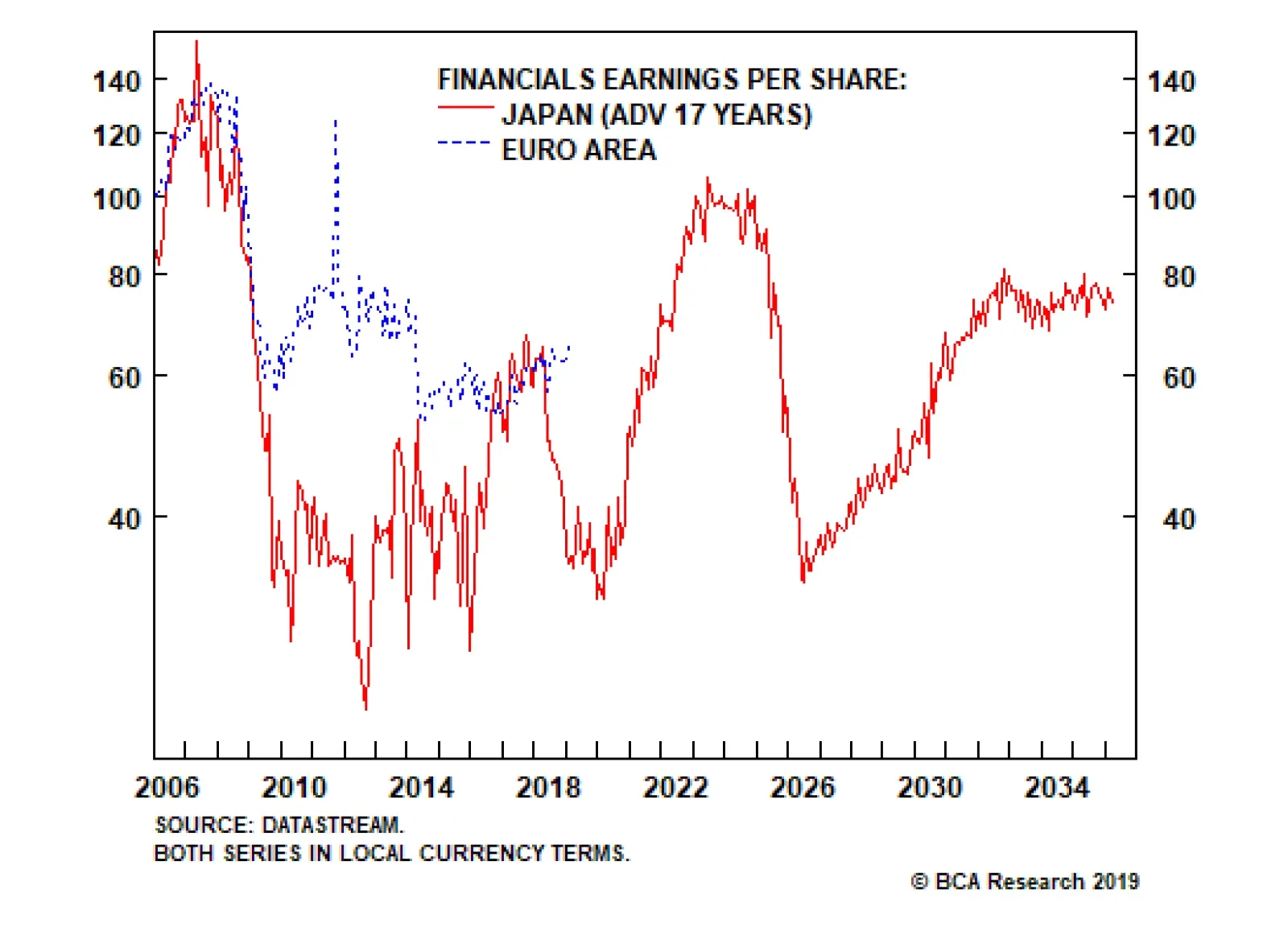
Japanese financial sector profits peaked in 1990 and stand at less than half that level today. Euro area financial sector profits peaked in 2007, and are tracking the Japanese experience with a 17-year lag. If euro area financial profits continue to follow in…