United States
BCA Research’s US Bond Strategy service still views December 2022 as the most likely liftoff date. The team is monitoring five factors to see if their forecast needs to be revised. 1. The Unemployment Rate: The Fed has officially pledged through its…

With 119 S&P 500 companies having reported Q3-2021 earnings, it’s time to take a pulse of the interim results. So far, the blended earnings growth rate is 34.8% while actual reported growth rate is 49.9%. The blended sales growth rate is 14.4%, while the actual reported rate is 16.6%. Analysts expected Q3-2021 earnings to be 6% below the Q2-2021 level. As of now, this quarter’s earnings are only 3% lower. Most of the companies that have reported are beating analysts’ forecasts are surprising to the upside. Currently, 83% of companies reported EPS above expectations, with five out of eleven sectors delivering an impressive 100% beat score. In terms of the magnitude of the beats, the overall number currently stands at 14% with Financials and Technology leading the pack. However, these results are bound to change as more companies report: less than 5% of the market cap has reported within the Energy, Materials, Real Estate, and Utilities sectors. The big theme for the current earnings season is input cost inflation. Many industrial giants, including Honeywell (HON), are complaining about supply-chain cost increases, and their potential adverse effect on margins. As a result, many companies are reducing guidance for the fourth quarter. So far, there are 59 positive pre-announcements, and 45 negative. On the bright side, the majority of companies are reporting that demand for their products remains strong, potentially offsetting some of the cost increases. This is especially the case with consumer demand: a few consumer staples companies, such as P&G, commented that their recent price hikes have not dampened demand for their products and have fortified their bottom line against rising costs. Bottom Line: The earnings season is gaining speed, and so far, it appears that Q3-2021 growth expectations are set at a low bar, that is easy to clear for most companies.
Chart
Highlights Treasuries: Bond investors should maintain below-benchmark portfolio duration and continue to short the 5-year note versus a duration-matched 2/10 barbell. For those investors who want to take an outright long position in US Treasuries, the 2-year Treasury note looks like the best security to choose. Municipal Bonds: This week we upgrade our recommended allocation to municipal bonds from overweight (4 out of 5) to maximum overweight (5 out of 5). Investors who can take advantage of the muni tax exemption should favor municipal bonds over Treasuries and over corporate bonds with the same credit rating and duration. In particular, we recommend that investors focus on long-maturity municipal bonds. Fed: Given our view that inflation will fall during the next 12 months, we still view December 2022 as the most likely liftoff date. However, we will continue to monitor our Five Factors For Fed Liftoff to see if our forecast needs to be revised. Feature
Chart 1
Our call for a bear-flattening of the US Treasury curve has worked out well during the past few weeks. Long-maturity Treasury yields have almost risen back to their March highs, and the short-end of the curve has also participated in the recent bout of selling (Chart 1). In light of these moves, it makes sense to re-evaluate our nominal Treasury curve positioning. First, we consider whether, at current yield levels, it still makes sense to run below-benchmark portfolio duration. Second, we consider whether our current recommended yield curve trade (short the 5-year note versus a duration-matched 2/10 barbell) remains the best way to extract returns from changes in the yield curve’s shape. The next section of this report answers these questions by looking at forecasted returns for different Treasury maturities across a variety of plausible economic and monetary policy scenarios. Later in the report we look at municipal bond valuation and provide a quick update on last week’s Fedspeak. Forecasting Treasury Returns
Chart 2
Three sources of Treasury bond return need to be considered when creating a forecast. Income Return: The return earned from the bond’s coupon payments. Rolldown Return: The return that a bond accrues simply by moving closer to its maturity date in an unchanged yield curve environment. Capital Gains/Losses: The return earned by a bond due to changes in the level and slope of the yield curve. We like to combine the income and rolldown return into one measure called “carry”. The carry can be thought of as the return an investor will earn in a specific bond if the yield curve remains unchanged throughout the investment horizon. Though carry is not the be all and end all of bond returns, it can be illuminating to look at the yield curve in terms of carry instead of the typical yield-to-maturity. Chart 2 shows the usual par coupon yield curve alongside the 12-month carry for each Treasury security. At present, the steepness of the 3-7 year part of the curve means that bonds of those maturities benefit a lot from rolldown. In fact, we see that a 7-year Treasury note will earn more than a 10-year Treasury note during the next 12 months if the curve remains unchanged. After calculating carry, the next step is to calculate capital gains/losses for each bond. To do this, we create some possible scenarios for future changes in the fed funds rate and assume that the yield curve moves to fully price-in that funds rate path over the course of a 12-month investment horizon.1 Next, we calculate the capital gains/losses for each bond based on the new shape of the yield curve in each scenario. Tables 1A-1D show the results from four different scenarios where the Fed starts to lift rates in December 2022. We then assume that the Fed will lift rates at a pace of 75-100 bps per year and that the funds rate will level-off at a terminal rate of either 2.08% or 2.58%. The 2.08% terminal rate corresponds to the median estimate of the long-run neutral fed funds rate from the New York Fed’s Survey of Market Participants. The 2.58% terminal rate corresponds to the median forecast from the Fed’s Summary of Economic Projections.2
Chart
Chart
Chart
Chart
The scenario shown in Table 1B is the closest to our base case. In this scenario, some short-maturity bonds deliver positive returns, but returns are negative for the 5-year maturity and beyond. Also, the 5-year note delivers the worst total return of all the maturities we examine. Unsurprisingly, expected returns for the longer maturities drop significantly if we raise our terminal rate assumption to 2.58% (Tables 1C & 1D). Therefore, any call to short the 5-year note versus the long-end relies on an assumption that the market will trade as though the terminal rate is closer to 2% than to 2.5% during the next 12 months. This is in line with our expectation. Finally, we observe that slowing our pace assumption from 100 bps per year to 75 bps raises expected returns across the board, but the 5-year still performs worse than the other maturities (Table 1A). Due to our expectation that inflation will fall during the next 12 months, a December 2022 liftoff remains our base case.3 However, the market has recently moved to price-in an earlier start to rate hikes. As of last Friday’s close, the fed funds futures curve was priced for liftoff in September 2022 and for a total of 49 bps of tightening by the end of 2022 (Chart 3). Chart 3Market Priced For September 2022 Liftoff
Market Priced For September 2022 Liftoff
Market Priced For September 2022 Liftoff
Tables 2A-2D incorporate these recent market moves into our forecast by looking at the same scenarios as in Tables 1A-1D but assuming a September 2022 liftoff instead of December. The results are not all that different. Expected returns are worse across the board, but the 5-year still looks like the worst spot on the curve unless the market starts to price-in a higher terminal rate.
Chart
Chart
Chart
Chart
Investment Conclusions Most of the scenarios we examined had negative expected returns for most maturities. We therefore still think it makes sense to keep portfolio duration low. Further, in every scenario the best expected returns can be found in the shorter maturities. In fact, the 2-year Treasury note offers positive returns in every scenario we examined. An outright long position in the 2-year Treasury note looks like a decent trade for investors forced to hold bonds. As for the yield curve, our results suggest that we should continue with our current positioning: short the 5-year note versus a duration-matched 2/10 barbell. The 5-year note performs worst in every scenario that assumes a 2.08% terminal rate. While it’s conceivable that investors will eventually push their terminal rate expectations higher, we think this is more likely to occur once the Fed has already lifted rates a few times. Bottom Line: Bond investors should maintain below-benchmark portfolio duration and continue to short the 5-year note versus a duration-matched 2/10 barbell. For those investors who want to take an outright long position in US Treasuries, the 2-year Treasury note looks like the best security to choose. The Duration Drift In Municipal Bond Valuations One under-discussed aspect of municipal bonds is that the securities tend to pay higher coupons than other bonds. That is, the bonds will often be issued with coupon rates well above prevailing yields. Investors therefore must pay a higher price to purchase the bonds, but they receive more return in the form of coupon payments. This feature of municipal bonds has important implications for how we should value them. For example, while the average maturity of the Municipal Bond index is much higher than the average maturity of the Treasury index, the muni index’s higher coupon rate makes its average duration significantly lower (Chart 4). This means that any valuation measure that compares a municipal bond’s yield with the yield of another bond with the same maturity will be unflattering for the muni. Chart 4Munis Pay High Coupons, Have Low Durations
Munis Pay High Coupons, Have Low Durations
Munis Pay High Coupons, Have Low Durations
Further, since Treasury securities and corporate bonds tend to issue at par, the coupon rates paid by those securities have fallen alongside yields during the past few decades. Meanwhile, municipal bond coupons have been relatively stable (Chart 4, panel 3). This means that, over time, municipal bond durations have fallen significantly compared to the durations of other US bond sectors. A fair valuation measure would compare municipal bond yields with equivalent-duration Treasury yields and that is exactly what we’ve done. Chart 5A shows the spread between General Obligation (GO) muni bond yields and equivalent-duration Treasury yields. Chart 5B shows the spreads expressed as percentile ranks. For example, a percentile rank of 50% means that the spread is at its historical median, a percentile rank of 10% means the spread has only been tighter 10% of the time. Chart 5AGO Muni/Treasury Spreads I
GO Muni/Treasury Spreads I
GO Muni/Treasury Spreads I
Chart 5BGO Muni/Treasury Spreads II
GO Muni/Treasury Spreads II
GO Muni/Treasury Spreads II
The first thing that jumps out from our analysis is that municipal bonds are not that expensive. Shorter-maturity spreads were tighter than current levels as recently as 2019/20 and the long-maturity (17-year+) spread is positive, despite the muni tax exemption. In terms of percentile rank, spreads for all GO maturity buckets are only just below the historical median. However, spreads traded much tighter prior to the 2008 financial crisis and it may not be reasonable to expect munis to return to those tight mid-2000 valuations. Charts 6A and 6B repeat the exercise from Charts 5A and 5B but for Revenue bonds instead of GOs. The message is similar. Muni valuations are not that stretched compared to history, and investors can earn a before-tax spread pick-up in munis versus Treasuries if they focus on the long maturities. Chart 6ARevenue Muni/Treasury Spreads I
Revenue Muni/Treasury Spreads I
Revenue Muni/Treasury Spreads I
Chart 6BRevenue Muni/Treasury Spreads II
Revenue Muni/Treasury Spreads II
Revenue Muni/Treasury Spreads II
In fact, municipal bonds offer a before-tax yield advantage versus Treasuries for Revenue bonds beyond the 12-year maturity point and for GO bonds beyond the 17-year maturity point. Further, the breakeven tax rate for 12-17 year GOs versus Treasuries is a mere 1% and the breakeven tax rate for 8-12 year Revenue bonds is only 8%. Investors facing a tax rate above the breakeven rate will earn an after-tax yield pick-up in munis versus duration-matched Treasuries (Table 3). Table 3Muni/Treasury And Muni/Credit Yield Ratios
The Best & Worst Spots On The Yield Curve
The Best & Worst Spots On The Yield Curve
Of course, municipal bonds also carry a small credit risk premium relative to duration-matched Treasuries. The GO and Revenue indexes have average credit ratings of Aa1/Aa2 and Aa3/A1, respectively, compared to a Aaa rating for US Treasuries. But we can control for credit risk as well by comparing municipal bonds to the US Credit Index and matching both the duration and credit rating. Even this comparison looks favorable for municipal bonds. Once again, long-maturity munis offer a before-tax yield advantage compared to credit rating and duration-matched US Credit. Meanwhile, breakeven tax rates for other maturities are low enough to attract most investors. Bottom Line: This week we upgrade our recommended allocation to municipal bonds from overweight (4 out of 5) to maximum overweight (5 out of 5). Investors who can take advantage of the muni tax exemption should favor municipal bonds over Treasuries and over corporate bonds with the same credit rating and duration. In particular, we recommend that investors focus on long-maturity municipal bonds, noting that the relatively low duration of these bonds makes them attractive relative to other bonds with similar risk profiles. Five Fed Factors A lot of Fedspeak hit the tape last week. Of particular interest were an interview with Chair Jay Powell on Friday and speeches by Fed Governors Randy Quarles and Chris Waller on Wednesday and Tuesday. One takeaway from their remarks is that a tapering announcement at the next FOMC meeting is very likely, with net asset purchases expected to hit zero by the middle of next year. The market, however, seems to have already taken the taper announcement on board. The more interesting aspects of the speeches were the discussions about how the Fed will decide when to lift rates and how elevated inflation readings may or may not influence that decision. We’ve noted in prior reports that five factors will determine when the Fed finally decides to lift rates, and last week’s comments gave us confidence that we’re on the right track. We run through our Five Factors For Fed Liftoff below, with some additional comments on why each factor is important (Table 4). Table 4Five Factors For Fed Liftoff
The Best & Worst Spots On The Yield Curve
The Best & Worst Spots On The Yield Curve
1. The Unemployment Rate The Fed has officially pledged through its forward guidance not to lift rates until “maximum employment” is reached. While the exact definition of “maximum employment” can be debated, there is widespread agreement that it includes an unemployment rate below its current adjusted level of 4.9%.4 More specifically, we inferred from the September Summary of Economic Projections that most FOMC participants view an unemployment rate of around 3.8% as consistent with “maximum employment” (Chart 7).5 Chart 7Defining "Maximum Employment"
Defining "Maximum Employment"
Defining "Maximum Employment"
We expect that the Fed will refrain from lifting rates until the unemployment rate reaches 3.8%. 2. Labor Force Participation We explored the debate about labor force participation in a recent report.6 In short, there are some policymakers who believe that “maximum employment” cannot be achieved until the labor force participation rate has returned to pre-COVID levels. There are others, however, who think that an aging population and the recent uptick in retirements make such a return impossible. Randy Quarles, for example: I expect that as conditions normalize, [the labor force participation rate] will pick up, but it is unlikely to return to its February 2020 level. One reason is that a disproportionate number of older workers responded to the initial shock of the COVID event by retiring, which may be an area where participation and employment struggle to retrace lost ground.7 In his speech, Governor Waller also mentioned “2 million jobs” that will be lost forever due to retirements.8 While many policymakers cite increased retirements as a reason why the overall labor force participation rate will remain permanently lower, there is much broader agreement that a reasonable definition of “maximum employment” should include the prime-age (25-54) labor force participation rate being much closer to its February 2020 level (Chart 7, bottom panel). We think the Fed will refrain from lifting rates until the prime-age (25-54) labor force participation rate is close to its February 2020 level. 3. Wage Growth Accelerating wages are a tried-and-true signal that the labor market is running hot. While wage growth is rising quickly right now (Chart 8), there is a strong sense that this is due to pandemic-related labor supply shortages and that wage growth will moderate as pandemic fears (and labor shortages) wane. Chart 8Wage Growth
Wage Growth
Wage Growth
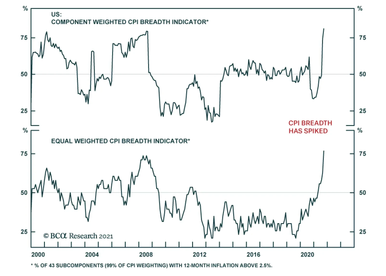
What will be more important is what wage growth looks like when the unemployment rate is close to the Fed’s target of 3.8%. At that point, accelerating wages will give the Fed a strong signal that a 3.8% unemployment rate really does constitute “maximum employment”. 4. Non-Transitory Inflation Of our five factors, this is admittedly the most difficult to pin down. However, Governor Quarles did a good job of explaining non-transitory inflation in last week’s speech: The fundamental dilemma that we face at the Fed now is this: Demand, augmented by unprecedented fiscal stimulus, has been outstripping a temporarily disrupted supply, leading to high inflation. But the fundamental productive capacity of our economy as it existed just before COVID – and, thus, the ability to satisfy that demand without inflation – remains largely as it was, constraining demand now, to bring it into line with a transiently interrupted supply, would be premature. Essentially, Quarles is saying that the Fed does not want to respond to a pandemic-related supply shock by lifting rates and curtailing aggregate demand. The Fed only wants to tighten policy if it sees an increase in broad-based inflationary pressures that will not be contained naturally by a return to more normal aggregate supply conditions. Accelerating wages would be one signal of such broad-based inflationary pressures, as would be measures of core inflation excluding those sectors that have been most impacted by the pandemic supply disruptions (Chart 9). Lastly, we could also look at indicators of inflation’s breadth across its different components, which have recently spiked to concerning levels (Chart 10). Chart 9Non-Covid Inflation
Non-Covid Inflation
Non-Covid Inflation
Chart 10CPI Breadth Has Spiked
CPI Breadth Has Spiked
CPI Breadth Has Spiked
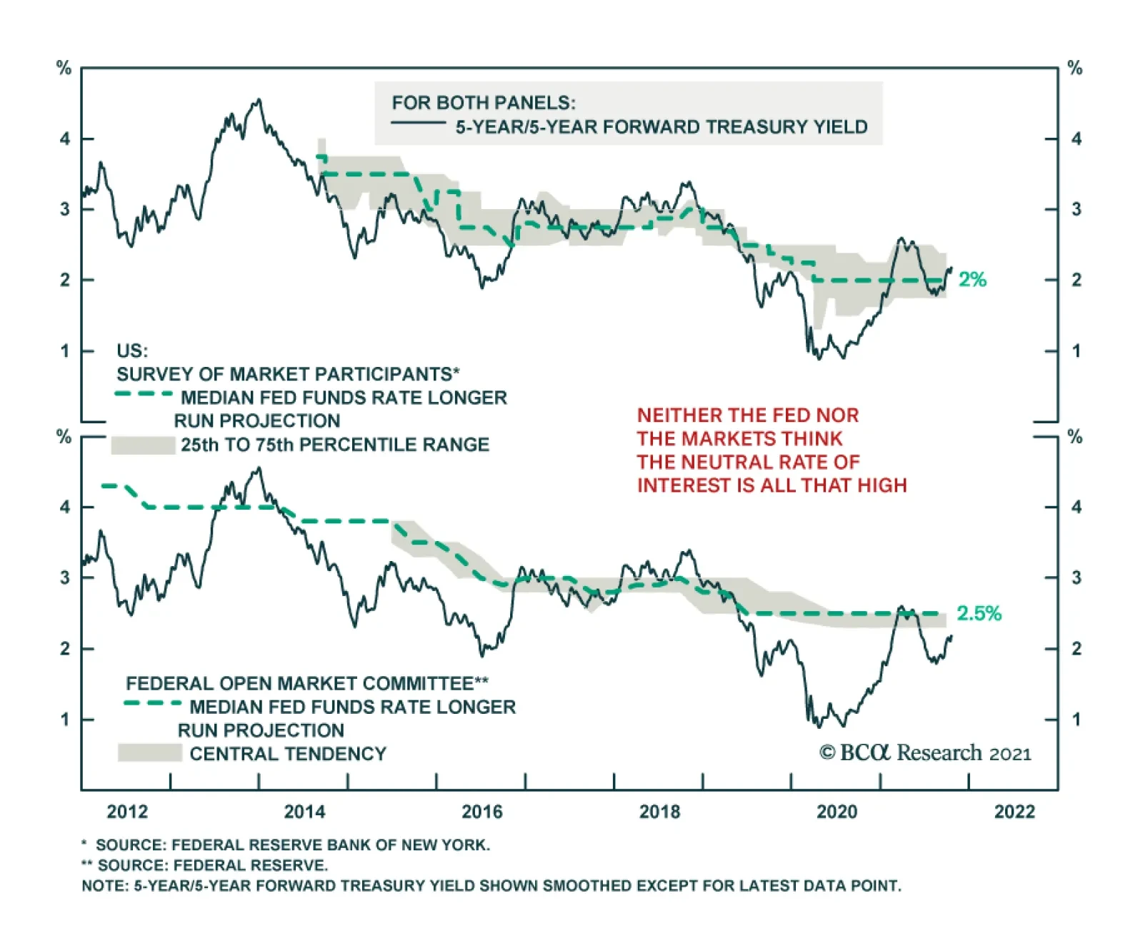
5. Inflation Expectations Inflation expectations are also critical to monitor. While all Fed participants seem to agree that inflation will fall during the next year, there is also widespread agreement that if high inflation causes inflation expectations to rise to uncomfortably high levels, then the Fed will be forced to act. Chris Waller: A critical aspect of our new framework is to allow inflation to run above our 2 percent target (so that it averages 2 percent), but we should do this only if inflation expectations are consistent with our 2 percent target. If inflation expectations become unanchored, the credibility of our inflation target is at risk, and we likely would need to take action to re-anchor expectations at our 2 percent target. At present, inflation expectations remain well-anchored near levels consistent with the Fed’s target (Chart 11). In particular, we like to track the 5-year/5-year forward TIPS breakeven inflation rate targeting a range of 2.3% to 2.5% as consistent with the Fed’s target. Incidentally, Governor Waller also flagged TIPS breakeven inflation rates as his “preferred” measure of inflation expectations in last week’s speech. Chart 11Inflation Expectations Remain Well-Anchored
Inflation Expectations Remain Well-Anchored
Inflation Expectations Remain Well-Anchored
The Fed will move much more quickly toward rate hikes if the 5-year/5-year forward TIPS breakeven inflation rate moves above 2.5%. Bottom Line: Given our view that inflation will fall during the next 12 months, we still view December 2022 as the most likely liftoff date. However, we will continue to monitor our Five Factors For Fed Liftoff to see if our forecast needs to be revised. Ryan Swift US Bond Strategist rswift@bcaresearch.com Footnotes 1 All of our scenarios use a 12-month investment horizon and assume a term premium of 0 bps. 2 In both cases we assume that the fed funds rate trades 8 bps above its lower-bound, as is currently the case. 3 Please see US Bond Strategy Weekly Report, “Right Price, Wrong Reason”, dated October 19, 2021. 4 We adjust the unemployment rate for distortions in the number of people employed but absent from work. Please see US Bond Strategy Weekly Report, “Overreaction”, dated July 13, 2021 for further details. 5 Please see US Bond Strategy Weekly Report, “Damage Assessment”, dated September 28, 2021. 6 Please see US Bond Strategy Weekly Report, “2022 Will Be All About Inflation”, dated September 14, 2021. 7 https://www.federalreserve.gov/newsevents/speech/quarles20211020a.htm 8 https://www.federalreserve.gov/newsevents/speech/waller20211019a.htm Recommended Portfolio Specification Other Recommendations Treasury Index Returns Spread Product Returns
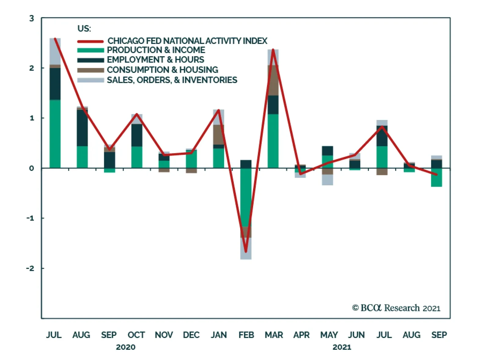
The Chicago Fed National Activity Index fell to a seven-month low of -0.13 in September, below the 0.2 consensus forecast. The index’s decline into negative territory corresponds with below-average growth for the US economy. Meanwhile, the August reading was…
BCA Research’s US Investment Strategy & US Equity Strategy services conclude that rising interest rates are not a good reason for equity investors to reduce their tech exposures. The empirical record poses several challenges to the conventional wisdom…
Highlights Contrary to popular belief, the correlation between changes in interest rates and equity returns is not fixed: Stock prices have generally risen as yields have fallen over the last four decades, but there is no rule that states equity returns and bond yields will be inversely related. Tech stocks’ tight recent inverse correlation with interest rates is a new phenomenon and we expect it will be temporary: Relative differences in earnings have driven relative returns since the global financial crisis and their mirror image correlation with interest rates was a pandemic anomaly that has already withered. Rising interest rates are not a good reason for equity investors to reduce their Tech exposures: The conventional wisdom is not always wrong, but it almost never generates alpha. In this case, we believe the crowd has fallen for a fleeting illusion that will not persist. Feature Table 1Lapping The Field
Tech Stocks And Interest Rates: Less Than Meets The Eye
Tech Stocks And Interest Rates: Less Than Meets The Eye
Perhaps nothing has lately generated more consensus agreement among equity strategists and other top-down observers than the claim that Tech stocks are particularly vulnerable to rising interest rates. Thanks to the Tech sector’s track record of generating outsized growth (Table 1), its future earnings streams are expected to be larger for longer than other sectors’, making them somewhat akin to long-maturity bonds from a duration perspective. Go-go growth stocks and Treasuries make for strange bedfellows, no matter how logical the earnings-stream reasoning may appear to be at first glance, and we view the application of duration concepts to equities as a stretch in any event. In this Special Report, we make the case that the recently observed tight inverse correlation between relative Tech sector performance and the 10-year Treasury yield is anomalous and should not be expected to persist. Right Church, Wrong Pew Duration is the weighted-average term to maturity of a bond’s cash flows and describes its price sensitivity to changes in interest rates. It is an essential feature of fixed income markets but attempts to extend the concept to equities necessarily fall flat. Bondholders receive interest and principal payments subject to a contractually fixed schedule that makes valuing a bond, especially one with negligible credit risk, a simple exercise in arithmetic. The present value of any bond (PV) is equal to the sum of its discounted series of cash flows, as in the equation
Chart
, where x = one of a series of n semi-annual payments, r = the discount rate and t = the time in years when the next payment will be received.
Chart 1
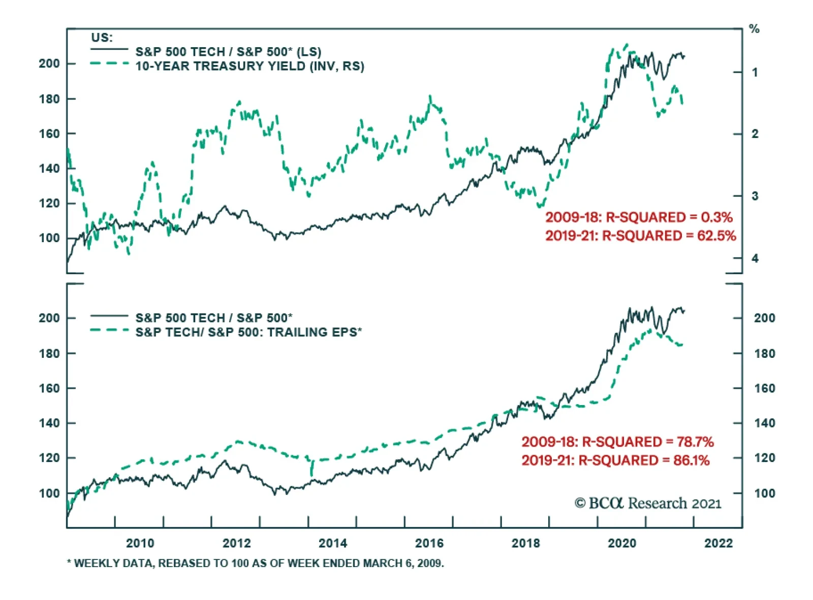
Assuming that all the interest payments and the principal payment will be received on time, the only variable term in the bond present value equation is the discount rate, r. As r appears solely in the denominator, a bond’s present value is inversely related to its moves. The cash streams accruing to stockholders are inherently unpredictable, however, and the present value of an equity interest is subject to fluctuations in the realized and estimated future values of x as well as changes in discount rate r. Forces that move r may or may not also move x and it is uncertain whether the numerator or denominator will exert a greater impact if they move together, as they might be expected to do in the case of the high-growth Tech sector. The explanatory power of changes in interest rates weakens as cash flow uncertainty increases. Month-over-month changes in the 10-year Treasury note yield1 explain virtually all the variation in one-month Bloomberg Barclays Treasury Index total returns (Chart 1, top panel). As cash flows become more uncertain with the introduction of modest credit risk, the correlation slips to -40% (Chart 1, middle panel). It weakens even further and flips its sign with equities, which have done better since the financial crisis when the 10-year yield rises than when it falls (Chart 1, bottom panel). Bottom Line: Duration is a metric for measuring bonds’ price sensitivity to changes in interest rates. Because of the uncertain nature of a company’s future cash flows and the multitude of independent variables that influence them, duration is an ill fit with equities. The Post-Crisis Experience The empirical record poses several challenges to the conventional wisdom about Tech stocks and interest rates, beginning with their desultory relationship in the first ten years following the financial crisis. From 2009 through 2018, changes in the 10-year yield are unable to explain any of the variability in relative Tech returns, though they exhibit a tight correlation beginning in 2019 (Chart 2). Tech stocks were utterly indifferent to the yield spikes of 2009 and 2010-11, as well as the sharp intervening decline in 2010, and only began to separate themselves from the field following the Brexit vote, outperforming the overall S&P 500 by 30 percentage points in just two years while the 10-year yield rose from 1.5% to 3%. They then proceeded to blow away the index as yields fell from 2.75% at the end of 2018 to 0.5% at the mid-2020 COVID bottom and have since fought the index to a draw despite a 100-basis point backup above 1.6%. Chart 2Nothing More Than A Lockdown Fling
Nothing More Than A Lockdown Fling
Nothing More Than A Lockdown Fling
In contrast to their all-over-the-map relationship with the level of interest rates, Tech stocks have exhibited a consistently tight fit with relative trailing earnings. A quantitatively inclined visitor from outer space viewing Chart 3 might reasonably conclude that relative Tech stock performance is fully explained by earnings, and all other variables are noise. The series have moved nearly in lockstep with each other and show that Tech’s relative trailing P/E multiple has been quite stable since the crisis. Until relative prices and relative earnings began heading in separate ways as the latter began to slip this Spring, Tech’s relative post-crisis outperformance had entirely been earned, not given. Chart 3Case Closed?
Case Closed?
Case Closed?
Multiples provide an opportunity for interest rate changes to re-enter the discussion. In a direct sense, Tech earnings are comparatively immune to moves in interest rates (the sector’s biggest constituents have immaterial amounts of debt and do not sell big-ticket items that have to be financed), though one might expect the price investors are willing to pay to claim a share of their comparatively backloaded future cash flows may well fluctuate with them. Chart 4, however, shows that the Tech sector’s relative forward multiple has not exhibited a consistent relationship with rates – the correlation between multiples and rates was positive and fairly strong from 2009 through 2018 but weakened and turned negative beginning in 2019. From 1995, when the forward multiple series began, through 2008 (not shown in the chart) the relationship was very weak and negative, generating an r-squared of just 1.4%. Chart 4Defying The Duration Intuition
Defying The Duration Intuition
Defying The Duration Intuition
The relationship between relative four-quarter forward earnings expectations and the 10-year yield sheds some light on how so many observers have been hoodwinked into mistaking correlation for causation. Excepting stretches at the beginning and the end of the 2009-2018 period, when relative forward estimates paid no heed to swings in interest rates, they exhibited a modest negative correlation with the 10-year yield (Chart 5). They moved together with one mind across all of 2020, but that solidarity appears anomalous when viewed against the entire post-crisis record generally and the years that bracket it specifically. In 2018-19, the two years preceding peak pandemic conditions, and 2021, the year following them, Tech’s relative forward earnings expectations have been flatly indifferent to the rate backdrop. Chart 5One-Off
One-Off
One-Off
We submit that the recently observed tight correlation between the 10-year yield and relative forward earnings expectations is an isolated pandemic phenomenon. As bond yields plunged in 2020 due to extraordinary monetary accommodation and fears of a worst-case economic outcome, Tech’s heavy concentration of pandemic winners shot the lights out in terms of actual and projected earnings. Away from the narrow 2020 sample, however, the other twelve years of post-crisis data suggest that there’s no relationship between forward earnings expectations and interest rates. Tech outearned the broader market at a steady rate for the ten years preceding the pandemic without regard for the rates market’s gyrations. Investment Implications Interest rates are a red herring for explaining variations in relative Tech stock performance. The ubiquity of the view that Tech stocks’ relative performance will be heavily influenced by changes in interest rates turns out to be another instance in which something everybody knows turns out not to be true. This finding does not make us Tech bulls; we think the big-picture backdrop is sufficiently mixed to justify our US Equity Strategy and Global Asset Allocation services’ neutral recommendations. We simply wanted to call out the flaws in a popular notion before it becomes even more entrenched. Changes in interest rates do not solely effect equity prices via a denominator effect. They impact the numerator as well. The numerator impacts are multifaceted and vary based on which factor comes to the fore in a given instance. They are much harder to anticipate and therefore hold much more promise for investors who can suss them out in advance. The denominator effect is immediately apparent to any undergraduate who has been introduced to the time value of money and therefore isn’t likely to generate alpha. What’s more, as Tech stocks’ relative performance history illustrates, the relationship between equities and rates is not fixed. The rise of globalization and the Fed’s post-Volcker inflation vigilance ushered in a multi-decade disinflationary trend that ultimately culminated in rampant deflation fears following the global financial crisis. Now that concerns about stagflation have shunted aside concerns about secular stagnation, investors are much less likely to cheer rate backups while wringing their hands over rate declines. As Arthur Budaghyan, BCA’s Chief Emerging Markets strategist, has written, the about-face in market perceptions of interest rates could flip the correlations between equity prices and interest rates from positive (stocks advance as rising interest rates are perceived as evidence of economic improvement) to negative (stocks fall when rates rise and rise when rates fall). Our colleague Jonathan LaBerge, managing editor of the Bank Credit Analyst, has noted that extended valuations increase growth stocks’ vulnerability to rising interest rates. We do not disagree, but they do not have all that much to fear if the backup in Treasury yields is in line with our US Bond Strategy service’s year-end 2021 and 2022 targets of 1.75% and 2-2.25%, respectively. Tech’s outperformance may well have run its course – relative performance is extended, the law of large numbers makes it increasingly difficult to sustain historic growth rates, the legal and regulatory outlook is darkening and a shift from pandemic winners to pandemic losers may be in train – but rising rates alone are not a good basis for trimming Tech exposures. Doug Peta, CFA Chief US Investment Strategist dougp@bcaresearch.com Footnotes 1 Duration measures a bond’s sensitivity to a parallel shift in the yield curve, but we use the 10-year Treasury yield as a proxy for the entire curve in our simple regressions of asset class returns against price changes.
BCA Research’s Global Investment Strategy service argues that the next step for inflation is likely down, even though the longer-term trend is to the upside. The path to structurally higher inflation is likely to be a bumpy one. The team has generally…
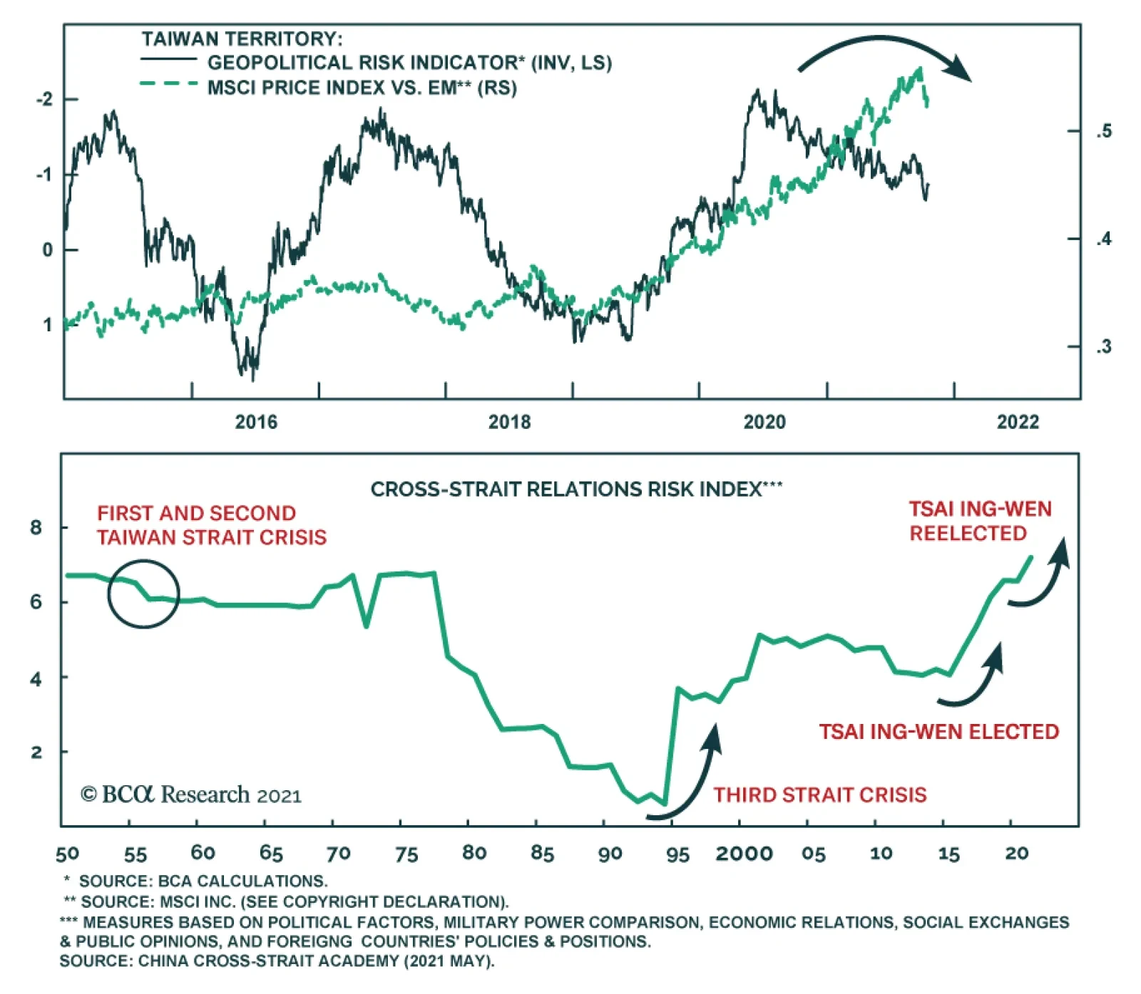
At a CNN town hall on Thursday President Biden stated that the US is committed to defending Taiwan[1] if China tried to attack it. The White House later clarified that there was no change in US policy towards Taiwan. Although the US supports Taiwan through…
Cybersecurity Primer
Cybersecurity Primer
In the coming weeks, we will continue our series of thematic Special Reports by conducting a “deep dive” analysis of cybersecurity stocks. This is a pervasive investment theme, and we recommend it as a new structural overweight. While cybersecurity is not new to the investment community, it is still in the early innings: The pandemic-driven shift to remote work, broad-based migration to cloud computing, development of the internet-of-things, and increasing geopolitical tensions create new targets for hackers who are after valuable data or just want to achieve maximum damage to the networks. With cybercrimes costing the world nearly $600 billion each year,1 and cyber-attacks increasing in number and sophistication, the global cybersecurity market is expected to grow from $125 billion in 2020 to $175 billion by 2024.2 Both large and small businesses are yet to fully implement cybersecurity defenses. According to a survey by Forbes magazine, 55% of business executives plan to increase their budgets for cybersecurity in 20213 aiming to prevent malicious attacks. These developments, are a boon for the cybersecurity stocks, making them an attractive long-term investment. In the upcoming Special Report, we will discuss the outlook and the key drivers of the industry, the types of cyber security defenses and companies behind them, and evaluate the fundamentals and valuation of our cyber security basket. We will draw investment conclusions to gauge the theme’s prospects as a tactical (three to six months investment horizon) investment. Bottom Line: Stay tuned for an upcoming Special Report on cybersecurity equities in the coming weeks. Top three cybersecurity ETFs by AUM are: CIBR, HACK, and BUG. Footnotes 1Mordor Intelligence, 2020. 2IDC, “Ongoing Demand Will Drive Solid Growth for Security Products and Services, According to New IDC Spending Guide,” Aug 13, 2020. 3Forbes, 2020
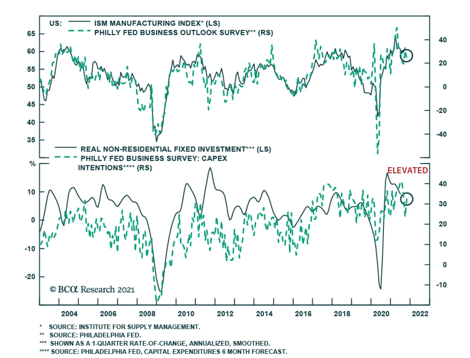
On the surface, the October Philadelphia Fed Business Outlook survey delivered a less optimistic message for the US economy. The Philly Fed index declined from 30.7 to 23.8 – falling slightly below expectations of 25.0. The 14-percentage point jump in the…