United States

Underweight (Upgrade Alert) We are currently underweight US banks, but the macro environment is changing and today we put this sub-sector on an upgrade alert looking to push it to a neutral allocation. The news on the buyback and dividend fronts is encouraging as banks will be allowed to resume their shareholder friendly activities that were halted last year due to the Fed’s Stress Test. Already, financials stocks are at the front of the pack with a roughly 3% total yield that is likely to increase further. Tack on the current search for yield environment, and the allure of financials equities becomes even more tempting. Bottom Line: We are putting banks on our upgrade alert watchlist. Please see an upcoming Strategy Report where we delve deeper into the buyback and dividend topics.
Buyback Revival?
Buyback Revival?

BCA Research’s US Political Strategy has just introduced its revised Quantitative Senate Election model. The six-variable model measures the probability of the incumbent party (Democratic Party) retaining the Senate in the 2022 midterm election. The…
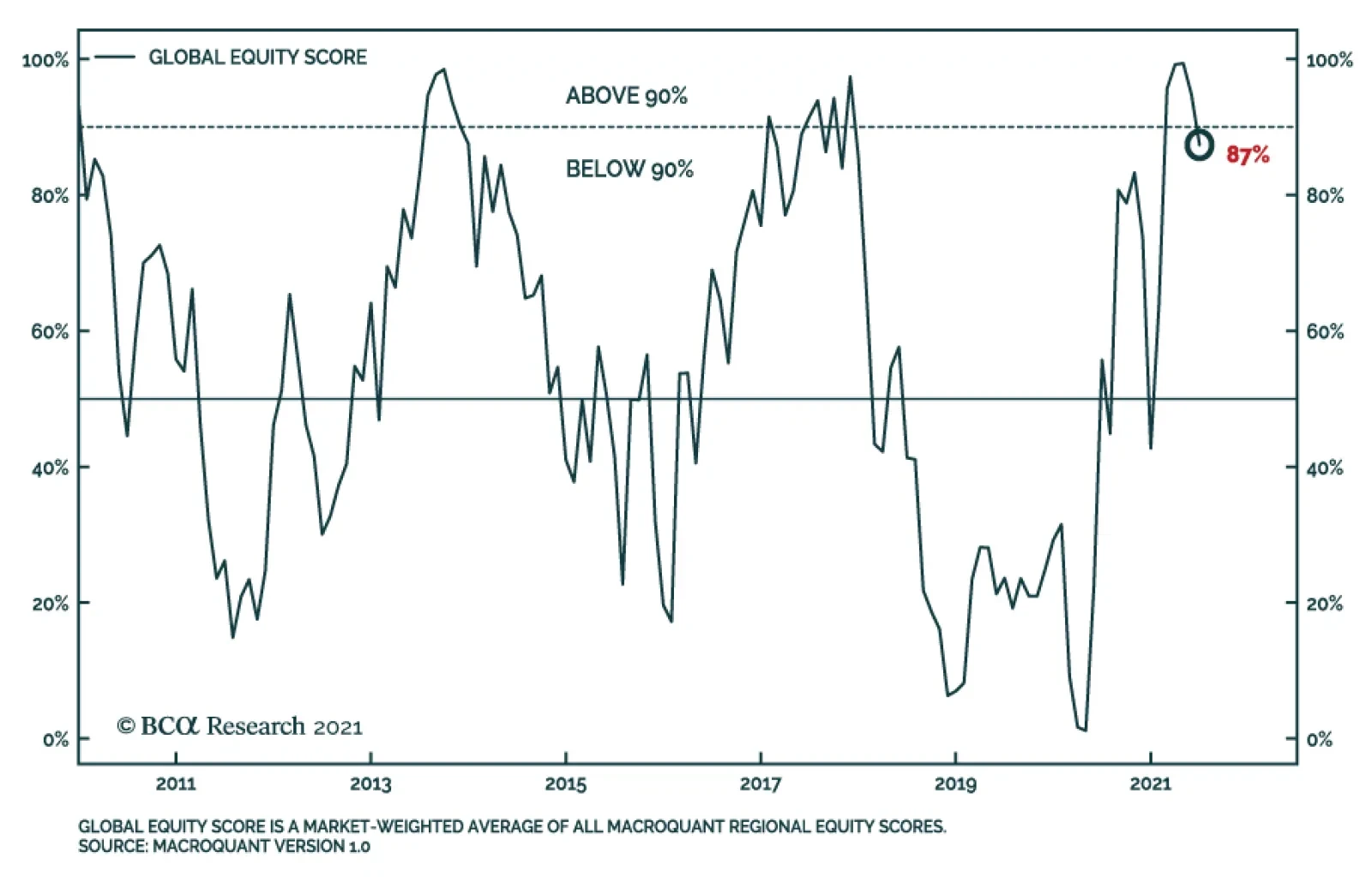
The MacroQuant global equity score is a market-weighted composite of all the regional equity scores within the model. It ranges between 0% and 100%, with 0% being most bearish and 100% being most bullish. Read the full details on MacroQuant in the recently…
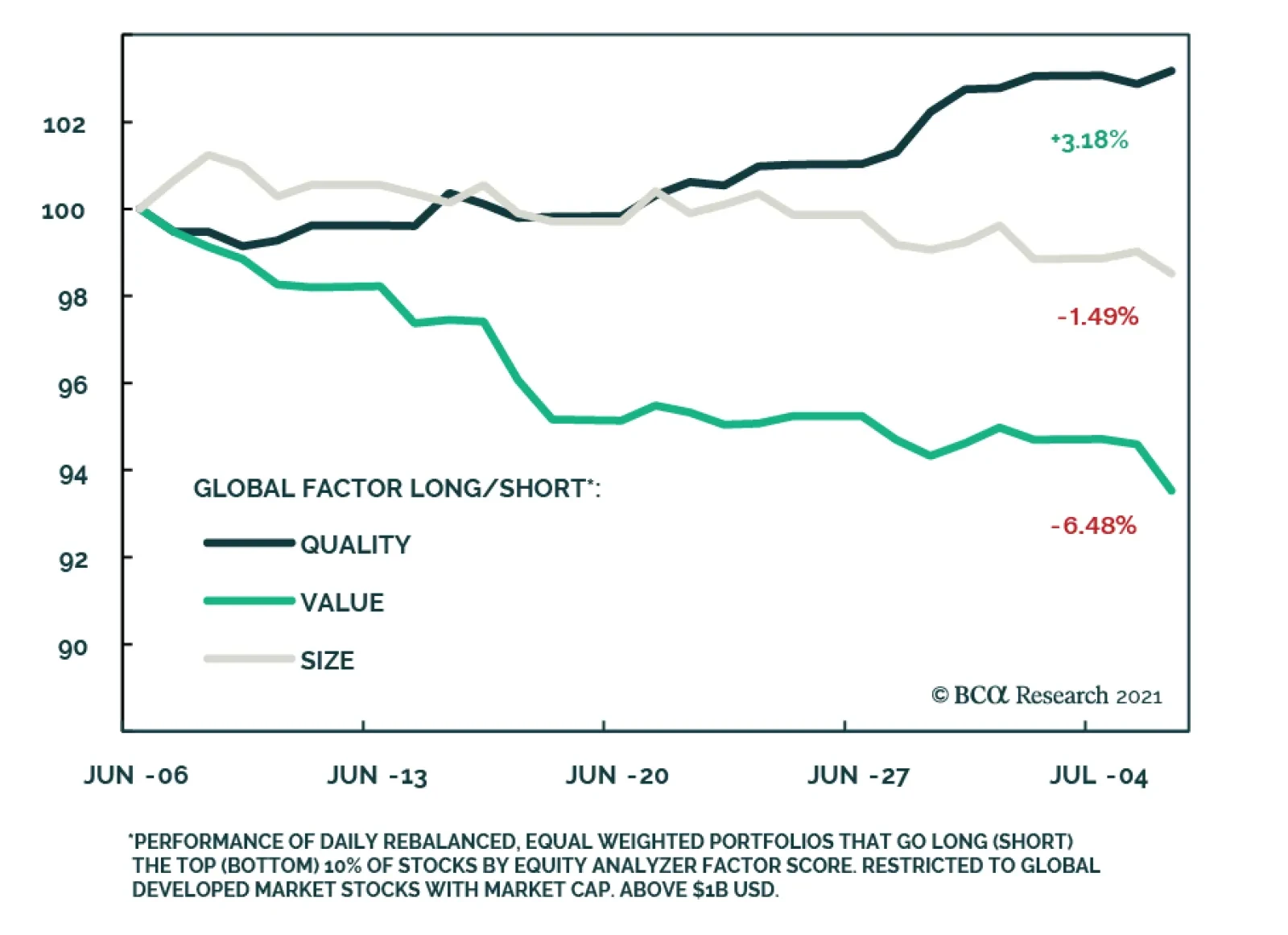
As recently highlighted by BCA Research’s US Equity strategists, we have seen a mid to short-term rotation out of cyclical sectors, notably materials, into growth sectors such as information technology. This has also occurred in line with a steady decrease in…
Highlights Complementing the US Political Strategy Quantitative Presidential Election Model, we introduce our revised Quantitative Senate Election Model. Our senate election model measures the probability of the incumbent party (Democratic Party) to retain the Senate in the 2022 midterm election. The model predicts that Democrats are slightly favored to retain control of the Senate, though it is too early to call, which in combination with the high likelihood that the GOP will retake the House, points to a US political gridlock from 2023 to 2025. The “Blue Sweep” policy setting will end as early as the end of the year as Democrats pass Biden’s signature legislation. Post-midterm gridlock implies that taxes unlikely to rise further from 2023 while spending will not be subjected to cuts. While markets will not be alarmed if growth keeps up, near term surprises from potential tax hikes, rate hikes, and China’s slowdown warrants a more defensive positioning. Feature 2020 was not only the year of a highly contested US Presidential election, but also a close-knit battle for control of the US Senate, which had 351 seats up for reelection. The Republican party initially retained control of the Senate at the start of 2021 and the 117th congress, but this was short-lived. The Democrats secured victories in both run-off triggered Senate races in the state of Georgia, putting them at an even 50-50 hold with Republicans in the Senate. The inauguration of Vice President Kamala Harris who too became the Senate President, was the tie breaker the Democrats needed to take control of the Senate, and ultimately secure a “blue sweep” of holding the House of Representatives, the Senate and the White House. We recently introduced BCA US Political Strategy readers to our quantitative presidential election model. If you have not yet read it, you can access it here. In this week’s report we introduce our US Political Strategy Senate election model. We acknowledged that it was still early days in the presidential election cycle when we published our presidential election model but there were however some interesting takeaways from an early model forecast. For control of the Senate, however, the cycle is much shorter, with voting of one third of the Senate taking place every two years. The mid-term elections of 2022 are not that far-out, and with 34 seats up for reelection, we believe that introducing our readers to our Senate election model now will start to provide valuable insight going forward. Like our presidential election model, our Senate election model is a state-by-state model that uses both economic and political variables to predict the number of seats the incumbent party will win in the 2022 Senate election. Our Senate model covers a large sample size, consisting of 19 Senate elections (1984 to 2020), across 50 states, amounting to 950 observations. The Six Variables Our Senate model is based off a Probit regression that produces a probability that each state will remain under the control of the incumbent party. The dependent variable (classified as “elected”) is stated as follows: 1 = Incumbent party wins the Senate election in each state; or 0 = Incumbent party did not win the Senate election in each state. This method allows us to measure the probability that a state with certain characteristics will fall into one of two categories above. We can then predict the probability of the incumbent party winning all the Senate seat/s in each of the 50 states (although this is only relevant to one-third of the states that have a Senate seat up for election in 2022). State economic health. Specifically, we use the Federal Reserve Bank of Philadelphia State Coincident Index for each of the 50 states. The coincident index combines four of a given state’s economic indicators to summarize current economic conditions in a single statistic. The four indicators are nonfarm payroll employment; average hours worked in manufacturing by production workers; the unemployment rate; and wage and salary disbursements plus proprietors' income deflated by the consumer price index (US city average). In other words, it captures job growth, manufacturing wages, joblessness, and real household income. The incumbent party’s margin of victory in previous Senate elections in each state Senate race. This is measured as the incumbent party’s share of the popular vote minus the non-incumbent party’s share. If the incumbent party failed to secure a solid win in each state in the previous Senate election, the probability of securing a solid win in the current election becomes smaller. Moreover, the larger the margin of victory in a previous Senate election race, the more likely that incumbent party will win re-election in said state. Net average approval level of the incumbent president in a Senate election year. This is the difference between the incumbent president’s approval and disapproval level in a Senate election year, from the start of the year up until the end of October of that year – taken as an average. Generic congressional ballot (net support rate). The generic congressional ballot asks people which party they are likely to vote for in Congress. We take the average net support rate in a Senate election year (that being whichever party leads the other in congressional ballot polling). Democrats are usually favored in congressional generic ballot voting, so the net rate is more predictive than the gross rate Dummy variable for congressional ballot. A dummy variable is assigned to variable number four. For example, dummy takes the value of 1 when Democrats have a positive net support rate in generic congressional ballot voting, and 0 when Republicans have a net positive support rate. We assign only one dummy variable to avoid a dummy variable trap.2 A “time for change” variable, a categorical variable indicating whether the incumbent party has controlled the Senate for three or more terms (six or more years). If the Senate has been controlled for three or more terms, the model will “punish” the incumbent party, as we would expect to see a change in control of the Senate the longer one incumbent party controls it. Democrats Retain Control Of The Senate As it stands, our election model predicts that Democrats will retain control of the Senate in 2022 (Chart 1). The Democrats are predicted to win 49 seats, a gain of one seat over the 2020 Senate election outcome,3 and when coupled with the two seats of Independent Senators, give them a majority of 51 seats. Chart 1Quant Model Gives Democrats 54% Chance Of Retaining The Senate
Introducing The US Political Strategy Quantitative Senate Election Model
Introducing The US Political Strategy Quantitative Senate Election Model
The additional seat for Democrats stems from our model allocating both North Carolina and Pennsylvania (which are currently occupied by Republicans) to the Democrats (+ two seats) and allocating one of Georgia’s seats occupied by Raphael Warnock4 back to Republican control. The Democrats overall probability of retaining control of the Senate is 54%, three percentage points higher than early market predictions (Chart 2). The market implied odds highlight another close battle between Democrats and Republicans to control the Senate in 2022. Chart 2Market Narrowly In Favor Of Democratic Senate Control
Introducing The US Political Strategy Quantitative Senate Election Model
Introducing The US Political Strategy Quantitative Senate Election Model
North Carolina is the only toss-up state,5 with a 51% chance of a Democratic victory. Pennsylvania will switch to Democrats and Georgia to Republicans. Note that North Carolina and Pennsylvania are both currently under Republican control. Both incumbents have decided not to run again. While both Georgia Senate run-off races were won by Democrats earlier this year, the sum of first-round voting in November 2020 was higher for Republican candidates than for Democrats. There was also extra-ordinary voter turnout in favor of Democrats for both run-offs, which ultimately played a big role in Democrats securing victory. Voter turnout was largely spurred on by voting against Republicans, and ultimately Donald Trump. This may not be the case come 2022, if turnout for Democrats is unmatched to 2020/2021. Our model’s prediction will evolve over time as new data become available, which could produce more toss-up states, or swing the prediction in favor of the opposing party. For now, the model provides us with a preliminary prediction as we draw nearer to the 2022 midterm elections. Senate Races Of Interest Comparing our model’s prediction to online betting markets, we group nine races into a category of “interest”. All nine races have varying degrees of probability for a Democratic win, ranging from approximately 30% to 60%. Five races are overestimated, and four races are underestimated by consensus (Chart 3). The remaining 25 races are decidedly in favor of either Democrat or Republican control, according to our model, so are therefore excluded from this analysis. Betting markets are overestimating Nevada, Arizona, Pennsylvania, Georgia, and Wisconsin, while underestimating New Hampshire, North Carolina, Florida and Ohio. Chart 3Senate Odds Compared With The Bookies
Introducing The US Political Strategy Quantitative Senate Election Model
Introducing The US Political Strategy Quantitative Senate Election Model
All nine of these races are precariously balanced, even at this stage of the mid-term election cycle. Small or local factors could ultimately decide the outcome. This is an important limitation on our macro model, highlighting our ultimate emphasis on qualitative analysis. For example, it is not at all clear that Democrats will win Georgia. Our model gives Democrats a 43% chance of victory. Betting markets are a lot more optimistic, penning a 55% chance of a Democratic win. But even by our model’s standard, Georgia remains a toss-up. Georgia may not be as close of a race as it was in 2020/2021, if voters are not as motivated as they were to vote Democrat. Will turnout be as large in 2022? That remains to be seen. One or two races with unique makeup can contribute to maintaining or shifting the balance of power in the Senate come 2022. Back Testing Our Model Our Senate model performs at an acceptable level during in-sample and out-sample back testing. For in-sample testing, we test our model over our entire sample period (1984 – 2020) and find that 74% of Senate elections (control of the Senate) are correctly predicted, with the model predicting the outcome of the last five Senate elections correctly (Chart 4). Chart 4In-Sample Back Testing Results
Introducing The US Political Strategy Quantitative Senate Election Model
Introducing The US Political Strategy Quantitative Senate Election Model
During out-sample back testing, we look at a sample period of 2000 – 2020, comprising of 11 Senate elections, where our model correctly predicts 73% of actual outcomes. The previous five Senate elections are predicted correctly too (Chart 5). Chart 5Out-Sample Back Testing Results
Introducing The US Political Strategy Quantitative Senate Election Model
Introducing The US Political Strategy Quantitative Senate Election Model
In comparison to our presidential election model, prediction accuracy of our Senate model is lower across its sample period. Predicting control of the Senate can sometimes be more uncertain than that of the White House. Both statistical and event based (Senate elections) reasons give way to a lower accuracy rate in this case. For example, there could be several idiosyncratic state-level variables not captured by our model, which could have played a leading role in determining any one state’s Senate election outcome over our sample period, and ultimately, control of the Senate. Where To From Here? In comparison to the presidential election cycle, we are a lot closer to election day. That means that Senate races will begin to heat up as we move closer toward November 8, 2022 – the date of the midterm elections. For now, our model ratifies the current control of the Senate, that is, Democratic. Our Model also suggests that come 2022, the Democrats will retain control of the Senate. But this is all but an early forecast. If any long-standing conclusion can be drawn right now, it is that the battle for control of the Senate in 2022 will be highly contested. From a qualitative point of view, our model may be overestimating the Democrats’ odds in 2022 as things stand today. Midterm elections have historically seen the sitting president’s party lose seats in the Senate and House of Representatives. We already expect Republicans to retake the House after a poor showing by Democrats in 2020. This narrative may play into the Republicans taking the Senate too – and is plausible given how closely the battle for the Senate is wound. But congressional approval has ticked higher lately under a Democratic run congress (Chart 6). Most likely, the American public have largely approved of COVID-19 government relief, and the Democrats will pass at least one more major piece of legislation covering infrastructure. Republicans are deeply divided, so there is some chance that they underperform in 2022. Nevertheless, the historical pattern clearly favors the opposition. The takeaway is to expect the GOP to retake the house but to monitor the Senate closely with both quantitative and qualitative tools. Chart 6US Public Approving Of Congress ?!?
Introducing The US Political Strategy Quantitative Senate Election Model
Introducing The US Political Strategy Quantitative Senate Election Model
Lastly, and importantly, we should note that in both the case of the presidential and Senate models, a probability between 50% and 55% for the incumbent party retaining control of the White House or Senate is indicative of an outcome “too close to call.” Both models are touting Democratic wins, but high conviction views about either the 2024 presidential election or 2022 Senate election are not warranted at this time. Investment Takeaway Unless 2022 is one of the rare cases of an incumbent party legislative victory after a national shock, like 1934 and 2002, Republicans will take the House at least. This is likely notwithstanding our model’s slight tilt in favor of Democrats in the Senate. This means that the “Blue Sweep” policy setting will cease as early as 2023, but de facto it would cease as early as the end of this year when Biden’s signature legislation is passed, since Congress will get little done in 2022. Our model suggests Republicans are slightly disfavored in the Senate. The truth is that as long as they gain one chamber of the legislature then US fiscal stimulus will virtually freeze. Taxes will no longer be able to rise from 2023 but spending will not be subject to cuts. Gridlock is reinforced by our presidential quant election model’s slightly higher odds of Democrats retaining the White House, which we think is underestimated at present. Hence Biden will retain veto power even if Democrats squander the Senate and House in 2022. Gridlock is thus looming from 2023 until at least 2025. The financial markets will not be alarmed by this forecast as long as growth keeps up. In the very near term, however, the clouds on the horizon of tax hikes, Fed rate hikes, and China’s tight-fisted economic policy pose rising headwinds to US equities in 2022 — and hence markets should respond negatively sooner than later. We are tactically growing more defensive. Guy Russell Research Analyst GuyR@bcaresearch.com Statistical Appendix Some clients may be curious as to how our US Political Strategy Senate election model differs from our Geopolitical Strategy model used in the 2020 elections, and where it has made improvements in its predictive accuracy. We discuss these improvements herein. Changes To The Geopolitical Strategy Senate Election Model A notable property in our dependent variable data requires a brief discussion. Our dependent variable classified as “elected” takes the form of a binary outcome. This data, however, is what’s called “unbalanced,” since incumbent Senators are re-elected approximately 80% of the time. This means that most outcomes in our dependent variable are coded as “1,” with fewer “0’s” because of the strong incumbency effect in Senate races. There are many data sets that exhibit this type of property, such as events like wars, vetoes, cases of political activism, or epidemiological infections, where non-events occur rarely. To alleviate this statistical property in the data, we estimate our model using a weighted maximum likelihood estimate as opposed to the ordinary maximum likelihood estimate usually used in a Probit regression.6 This method assigns more weighting to the unbalanced data, or what is known theoretically as “rare event” data, to aid the Probit regression in assigning higher probabilities to “0” outcomes. Through this process, we effectively deal with our unbalanced dependent variable data. The last update to the BCA Geopolitical Strategy Senate election model was published on January 6, 2021. Our model suggested that Republican’s would retain control of the Senate. Our model was limited in dealing with a unique twin Georgia run-off race that ultimately swung Senate control into the hands of the Democrats. The Geopolitical Strategy, which we will refer to as the 2020 model, only missed the Republican victory in Maine, but correctly predicted losses in Arizona and Colorado. The model missed both Georgia races, signaling they would remain red states – this was proven otherwise. Also, our model has become a better predictor in terms of in and out-sample forecasting (compared to our 2020 model). The 2022 version correctly predicts 74% (vs 72%) of in-sample and 73% (vs 70%) of out-sample outcomes. Methodology And Variables Our Senate model retains the methodology and suite of economic and political variables used in the model we first introduced in 2020. For long-time clients and those who are new to the US Political Strategy and Geopolitical Strategy service, the first version of our model can be found here. The one and only economic variable is now transformed by a six-month change to each state’s coincident index, capturing the improvement or deterioration of the state’s economy. The six-month change results in the best statistical fit for the overall model this time round. In the 2020 model, we transformed the variable by a three-month change. A fast-changing economic environment coupled with a then-higher statistical impact in our model led us to this decision. We still weight the transformation of our economic variable in the same manner as we did in last year’s updated model. We take a weighted average of the six-month change of all the monthly state coincident indices in the term preceding a Senate election. Later months are weighted heavier than earlier months as the most recent context will have a greater impact on voter opinion in the election. In terms of our political variables, they all remain the same as the 2020 model. Model Performance Classification The 2022 model correctly classifies predicted outcomes at a rate of exactly 81%. That is, when the model makes a prediction of a certain state’s Senate election outcome from 1984-2020, it is correct 81% of the time. This level of classification is higher than our 2020 model, which classified outcomes at a rate of 79% (Table 1). Table 1New Model Classifies Outcomes At A Higher Rate …
Introducing The US Political Strategy Quantitative Senate Election Model
Introducing The US Political Strategy Quantitative Senate Election Model
Sensitivity And Specificity – Receiver Operating Characteristic Curve A Receiver Operating Characteristic (ROC) curve is a performance measurement for classification problems of binary modelled outcomes, among others. An ROC curve tells us how much the model is capable of distinguishing between classes. In our case, we have two classes: the dependent variable (classified as “elected”) is stated as 1 = Incumbent party wins the Senate election in each state; or 0 = Incumbent party did not win the Senate election in each state. The higher the area under the curve (AUC), the better our model is at predicting 0 classes as 0 and 1 classes as 1. A robust model has an AUC near to one. A poor model has an AUC near to zero, which means it has the worst measure of classifying classes correctly, labelling zeros as ones and vice versa. In fact, at a level of zero AUC, the model is reciprocating incorrect classes by predicting zeros as ones and ones as zeros. Statistically, more AUC means that the model is identifying more true positives while minimizing the number/percent of false positives. Chart 7Receiver Operating Characteristic Curve Of 2022 Model
Introducing The US Political Strategy Quantitative Senate Election Model
Introducing The US Political Strategy Quantitative Senate Election Model
Table 2… Is A Better Fit …
Introducing The US Political Strategy Quantitative Senate Election Model
Introducing The US Political Strategy Quantitative Senate Election Model
The ROC curve for our 2022 model has an AUC of 0.9609 (Chart 7), a higher AUC than our 2020 model (Table 2). This means that the true positive rate for classifying outcomes is high and the false positive rate is low, improving on our model’s robustness. F1 Scores A final grading of the 2022 model is by means of the F1 score. The F1 score is a measurement that considers both precision (specificity in the above ROC curve) and recall (sensitivity in the above ROC curve) to compute the score. The F1 score can be interpreted as a weighted average of the precision and recall values, where an F1 score reaches its best value at 1 and worst value at 0. The 2022 model produces a higher F1 score compared to our 2020 model (Table 3). Table 3… And Is More Accurate Than The 2020 Model
Introducing The US Political Strategy Quantitative Senate Election Model
Introducing The US Political Strategy Quantitative Senate Election Model
Considering the improvement in forecast accuracy and overall better model specification over our 2020 model, we accept our 2022 model as our new base case Senate election model, premised on its improvement in accuracy at predicting election outcomes in the past, as well as its ability to correctly classify outcomes as they were realized. Appendix Tables Table A1USPS Trade Table
Introducing The US Political Strategy Quantitative Senate Election Model
Introducing The US Political Strategy Quantitative Senate Election Model
Table A2Political Risk Matrix
Introducing The US Political Strategy Quantitative Senate Election Model
Introducing The US Political Strategy Quantitative Senate Election Model
Chart A1Presidential Election Model
Introducing The US Political Strategy Quantitative Senate Election Model
Introducing The US Political Strategy Quantitative Senate Election Model
Table A3APolitical Capital: White House And Congress
Introducing The US Political Strategy Quantitative Senate Election Model
Introducing The US Political Strategy Quantitative Senate Election Model
Table A3BPolitical Capital: Household And Business Sentiment
Introducing The US Political Strategy Quantitative Senate Election Model
Introducing The US Political Strategy Quantitative Senate Election Model
Table A3CPolitical Capital: The Economy And Markets
Introducing The US Political Strategy Quantitative Senate Election Model
Introducing The US Political Strategy Quantitative Senate Election Model
Table A4Political Capital Index
Introducing The US Political Strategy Quantitative Senate Election Model
Introducing The US Political Strategy Quantitative Senate Election Model
Footnotes 1 Two of which were open Senate seats for the state of Georgia. 2 A dummy variable trap is a scenario in which the independent variables are multicollinear — a scenario in which two or more variables are highly correlated; or, in simple terms, in which one variable can be predicted from the others. To avoid such a trap, we must exclude one of the categorical variables. Since there are two categorical variables that can be represented here (Republican or Democrat), we use k-1 (where k = the number of categorical variables). 3 In reference to the Senate election outcome after the Georgia run-off races which concluded in early January 2021. 4 This seat formed part of the 2020 special Senate election race which was decided by a run-off election between Raphael Warnock and Kelly Loeffler. The seat was always up for reelection in 2022 no matter which party won it in the 2020 special election. 5 Toss-ups are defined as having a probability between 45% and 55% according to our model. 6 Weighted maximum likelihood estimation is a reasonable approach in dealing with dependent variables that show significant imbalance in their data set. See: King, G. and Zeng, L., 2001. Logistic regression in rare events data. Political analysis, 9(2), pp.137-163.
One Market To Rule Them All
One Market To Rule Them All
The bond market continues to dictate the pace for the SPX and relative sector performance. The 30-year US Treasury yield retraced nearly half a percent from the mid-March peak triggering a US equity market rotation from cyclical and value sectors like materials, into growth sectors such as technology. AMZN alone moved more than 3% yesterday breaking out to fresh all-time highs signaling continued outperformance of growth stocks, while more value sectors lag behind (see chart). With growth rolling over and the Fed staying pat despite a slightly more hawkish stance, we expect the rates market to remain range bound for a while longer, further supporting a strong run of growth stocks in general, and tech in particular. Bottom Line: The rotation trade into growth at the expense of value has more room to run.
GFIS Model Bond Portfolio Q2/2021 Performance Review & Current Allocations: Hitting A Few Roadblocks
Highlights Q2/2021 Performance Breakdown: Our recommended model bond portfolio underperformed the custom benchmark index by -6bps during the second quarter of the year. Winners & Losers: The government bond side of the portfolio underperformed by -21bps, led overwhelmingly by our underweight to US Treasuries (-18bps). Spread product allocations outperformed by +15bps, primarily due to overweights on US high-yield (+11bps) and US CMBS (+3bps). Portfolio Positioning For The Next Six Months: We are maintaining an overall below-benchmark portfolio duration stance, against a backdrop of persistent above-trend global growth and a highly stimulative fiscal/monetary policy mix. We are maintaining a moderate overweight to global spread product versus government debt, concentrated on an overweight to US high-yield where valuations look the least stretched. We are making two changes to the portfolio allocations heading into Q3: shifting the Treasury curve exposure to have more of a flattening bias, while downgrading EM USD-denominated corporates to neutral. Feature The trend in global bond yields so far in 2021 has been a tale of two quarters. The first three months of the year saw a surge in yields worldwide on the back of rapidly improving economic data, the rollout of COVID-19 vaccines and supply squeezes triggering rapid increases in inflation. During the second three months of the year, however, global yields drifted a bit lower in response to more mixed economic data, the spread of the Delta variant and slightly hawkish shifts from a few key central banks – most notably, the Fed – even with economic confidence measures remaining upbeat across the developed economies. The decline in yields has not been seen across the maturity spectrum, though. The yield-to-maturity of the Bloomberg Barclays Global and US Treasury 10+ year indices fell by -12bps and -30bps, respectively, from recent peaks. At the same time, shorter term bond yields have been relatively stable as central banks continue to signal that interest rate hikes are still well off into the future. In contrast to government bonds, credit markets have remained calm with spreads tight for developed market corporates and emerging market (EM) debt. With that in mind, we present our quarterly review of the BCA Research Global Fixed Income Strategy (GFIS) model bond portfolio during the second quarter of 2021. We also present our recommended positioning for the portfolio for the next six months (Table 1), as well as portfolio return expectations for our base case and alternative investment scenarios. The latter half of 2021 should prove to be even more challenging for bond investors, who must disentangle less consistent messages across countries on the Delta variant, vaccinations, inflation and the outlook for both monetary and fiscal policy. Table 1GFIS Model Bond Portfolio Recommended Positioning For The Next Six Months
GFIS Model Bond Portfolio Q2/2021 Performance Review & Current Allocations: Hitting A Few Roadblocks
GFIS Model Bond Portfolio Q2/2021 Performance Review & Current Allocations: Hitting A Few Roadblocks
As a reminder to existing readers (and to new clients), the model portfolio is a part of our service that complements the usual macro analysis of global fixed income markets. The portfolio is how we communicate our opinion on the relative attractiveness between government bond and spread product sectors. We do this by applying actual percentage weightings to each of our recommendations within a fully invested hypothetical bond portfolio. Q2/2021 Model Bond Portfolio Performance: Mixed Returns Chart 1Q2/2021 Performance: Credit Gains & Duration Losses
Q2/2021 Performance: Credit Gains & Duration Losses
Q2/2021 Performance: Credit Gains & Duration Losses
The total return for the GFIS model portfolio (hedged into US dollars) in the second quarter was +1.13%, slightly underperformed the custom benchmark index by -6bps (Chart 1).1 In terms of the specific breakdown between the government bond and spread product allocations in our model portfolio, the former generated -21bps of underperformance versus our custom benchmark index while the latter outperformed by +15bps. We have remained significantly underweight US Treasuries and positioned for a bearish steepening of the US Treasury curve since just before last year's US presidential election. That tilt was a big contributor to the excess return of the portfolio in Q1 (+63bps) that was partially given back (-18bps) in Q2 as longer maturity Treasury yields fell during the quarter. Our inflation-linked bond allocations in the US and Europe (+5bps) helped mitigate the loss on the government bond side from our below-benchmark duration stance and general curve steepening bias in most countries in the portfolio (Table 2). Table 2GFIS Model Bond Portfolio Q2/2021 Overall Return Attribution
GFIS Model Bond Portfolio Q2/2021 Performance Review & Current Allocations: Hitting A Few Roadblocks
GFIS Model Bond Portfolio Q2/2021 Performance Review & Current Allocations: Hitting A Few Roadblocks
The sum of excess returns during the quarter from countries that we overweighted (Germany, France, Italy, Spain, and Japan) was zero. Improving growth momentum and stronger economic confidence helped push yields higher in those countries. Therefore, those positions could not offset the losses from the underweight to US Treasuries. We did make two shifts in the country allocation within the government bond portion of the portfolio during Q2, downgrading Canada to underweight on April 20 and upgrading Australia to overweight on June 9. Neither change meaningfully contributed to the return of the portfolio. Meanwhile, our moderate overall overweight tilt on spread product versus government bonds fueled the outperformance from the credit side of the portfolio, led by US high-yield (+11bps) and US CMBS (+3bps). Overall gains from spread product were impressive in both USD-hedged total return terms (+95bps) and relative to our custom benchmark (+15bps), despite spreads entering Q2 at fairly tight levels. In the second quarter, improving economic confidence and easing credit conditions allowed spreads to narrow even further for corporate debt in the US and Europe, as well as for EM USD-denominated credit. The bar charts showing the total and relative returns for each individual government bond market and spread product sector are presented in Charts 2 & 3. Chart 2GFIS Model Bond Portfolio Q2/2021 Government Bond Performance Attribution
GFIS Model Bond Portfolio Q2/2021 Performance Review & Current Allocations: Hitting A Few Roadblocks
GFIS Model Bond Portfolio Q2/2021 Performance Review & Current Allocations: Hitting A Few Roadblocks
Chart 3GFIS Model Bond Portfolio Q2/2021 Spread Product Performance Attribution By Sector
GFIS Model Bond Portfolio Q2/2021 Performance Review & Current Allocations: Hitting A Few Roadblocks
GFIS Model Bond Portfolio Q2/2021 Performance Review & Current Allocations: Hitting A Few Roadblocks
Biggest Outperformers: Overweight US high-yield: Ba-rated (+5bps), B-rated (+4bps), and Caa-rated (+3bps) Overweight US TIPS (+4bps) Overweight US CMBS (+3bps) Overweight Euro Area high-yield (+1bps) Biggest Underperformers: Underweight US Treasuries with a maturity greater than 10 years (-17bps), Underweight US Treasuries with a maturity between 7 and 10 years (-3bps) Underweight US Treasuries with a maturity between 5 and 7 years (-2bps) Underweight EM USD sovereigns (-1bps) Underweight UK GIlts with a maturity greater than 10 years (-1bps) Chart 4 presents the ranked benchmark index returns of the individual countries and spread product sectors in the GFIS model bond portfolio for Q2/2021. Returns are hedged into US dollars (we do not take active currency risk in this portfolio) and adjusted to reflect duration differences between each country/sector and the overall custom benchmark index for the model portfolio. We have also color coded the bars in each chart to reflect our recommended investment stance for each market during Q2 (red for underweight, dark green for overweight, gray for neutral). Chart 4Ranking The Winners & Losers From The GFIS Model Bond Portfolio Universe In Q2/2021
GFIS Model Bond Portfolio Q2/2021 Performance Review & Current Allocations: Hitting A Few Roadblocks
GFIS Model Bond Portfolio Q2/2021 Performance Review & Current Allocations: Hitting A Few Roadblocks
Ideally, we would look to see more green bars on the left side of the chart where market returns are highest, and more red bars on the right side of the chart were returns are lowest. In Q2, the picture on that front was mixed. We were only neutral some of the biggest outperformers like UK Gilts (+312bps in USD-hedged duration-matched total return terms) and investment grade credit in the US (+430bps) and UK (+231bps). Our relative value allocation within EM, overweight corporates (+430bps) versus sovereigns (+527bps), also underperformed during Q2. We remained overweight government debt markets in the euro area which were the worst performers during the quarter (Germany: -25bps, Spain: -59bps, Italy: -67bps, and France: -83bps). The news was better on the credit side, where our significant overweight to US high-yield (+146bps) was a big positive contributor, as were overweights to US CMBS (+137bps) and euro area high-yield (+92bps). Bottom Line: Our model bond portfolio slightly underperformed its benchmark index in the second quarter of the year by -6bps – a negative result mainly driven by our underweight allocation to the US Treasury market but with an overweight to US high-yield providing a meaningful offset. Future Drivers Of Portfolio Returns & Scenario Analysis Looking ahead, the performance of the model bond portfolio will continue to be driven primarily by swings in global government bond yields, most notably US Treasuries. Our most favored cyclical indicators for global bond yields are still, in aggregate, signaling more upside potential over at least the next six months, although the nature of the signal is changing (Chart 5). Our Global Duration Indicator, comprised of leading economic indicators and measures of future economic sentiment, remains elevated but appears to have peaked. At the same time, the global manufacturing PMI, which typically leads global real bond yields by around six months, continues to climb to new cyclical highs. This suggests that the recent downdraft in global real bond yields could prove to be short-lived. Our Global Central Bank Monitor is climbing steadily, indicating greater upward pressure on bond yields from the combination of strong growth, rising inflation and loose financial conditions. Admittedly, bond yields are lagging the upward trajectory implied by the Monitor with central banks deliberately responding far more slowly to the cyclical pressures that would have triggered bond-bearish monetary tightening in the past. Nonetheless, the Monitor, the Global Duration Indicator and the global manufacturing PMI and all sending the same message – global bond yields remain too low, suggesting a below-benchmark overall portfolio duration stance remains appropriate. With regards to country allocation within the government bond side of our model portfolio, we continue to overweight countries where central banks are less likely to begin normalizing pandemic-era monetary policy quickly (Germany, France, Italy, Spain, Japan, Australia), while underweighting countries where normalization is expected to begin within the next 6-12 months (the US and Canada). We remain neutral the UK, although we have them on “downgrade watch” until there is greater clarity on how severely the spread of the Delta variant is impacting UK growth. The US remains the biggest underweight. The modestly hawkish turn by the Fed at the June FOMC meeting likely marked the end of the cyclical bear-steepening trend of the US Treasury curve. A full-blown turn to a bear-flattening of the US curve will be slow to develop, but we fully expect the cyclical pressures that drove the underperformance of longer-maturity US Treasuries over the past year to begin leaking into shorter-maturity bonds. That trend already appears to be underway with 5-year US yields starting to drift upward at a faster pace compared to other developed market peers (Chart 6). Chart 5Cyclical Indicators Suggest Global Yields Still Have More Upside
Cyclical Indicators Suggest Global Yields Still Have More Upside
Cyclical Indicators Suggest Global Yields Still Have More Upside
Chart 6UST Underperformance Will Shift To Shorter Maturities
UST Underperformance Will Shift To Shorter Maturities
UST Underperformance Will Shift To Shorter Maturities
This leads us to make a change to our model portfolio allocations this week, reducing the exposure to the belly of the US Treasury curve (the 3-5 year and 5-7 year maturity buckets), while modestly increasing the allocation to the 7-10 year bucket. To neutralize the duration-extending implication of that marginal shift, we added a new allocation to US Treasury bills, thus turning this US Treasury shift into a “butterfly” trade, essentially selling the 5-year bullet for a cash/10-year barbell. Longer-term Treasury yields, however, are still in the process of working off an oversold condition that developed in Q1 (Chart 7). Duration positioning remains quite short, according to the JP Morgan survey of bond investors, while speculators are still working off a huge net short position in 30-year Treasury futures according to data from the CFTC. We anticipate that it will take another month or two to work off such an extreme oversold condition for US Treasuries, based on similar episodes over the past two decades. After that, longer-maturity Treasury yields will begin to begin climbing again, to the benefit of the US underweight (and below-benchmark duration stance) in our model portfolio. Chart 7Longer-Maturity USTs Working Off Oversold Condition
Longer-Maturity USTs Working Off Oversold Condition
Longer-Maturity USTs Working Off Oversold Condition
Chart 8A Sharply Diminished Impulse From Global QE
A Sharply Diminished Impulse From Global QE
A Sharply Diminished Impulse From Global QE
Outside the US, the bond-friendly impact of quantitative easing programs is fading, on the margin, with the growth of central bank balance sheets slowing (Chart 8). While outright tapering of bond buying has only occurred in Canada and the UK (within our model bond portfolio universe), we expect the Fed to begin tapering in early 2022. Financial stability concerns are expected to play an increasingly important role in future tapering decisions, with house prices booming in many countries, most notably Canada which supports our underweight stance on Canadian government debt. Australia is the notable exception to this trend towards slowing balance sheet growth, with the Reserve Bank of Australia (RBA) maintaining a healthy pace of bond buying given underwhelming realized inflation. The recent wave of COVID-19 cases, which has left half of Australia under lockdowns that were largely avoided in 2020, will ensure that the RBA stays dovish for longer, to the benefit of our overweight stance on Australian government bonds. We continue to see the overall dovish stance of global central bankers as being conducive to the outperformance of inflation-linked bonds versus nominal government debt. However, inflation breakevens in most countries have largely completed the rebound from the depressed levels reached during the 2020 COVID-19 global recession. Our Comprehensive Breakeven Indicators combine three measures to determine the upside potential for 10-year inflation breakevens: the distance from fair value based on our models, the spread between headline inflation and central bank target inflation, and the gap between market-based and survey-based measures of inflation expectations. Those indicators suggest that the most attractive markets to position for further upside potential for breakevens are in Italy and France, with breakevens looking more stretched in the US, Canada and Australia (Chart 9). On the back of this, we are maintaining our allocations to inflation-linked bonds in the euro area in our model portfolio. Chart 9Less Scope For Wider Global Inflation Breakevens
Less Scope For Wider Global Inflation Breakevens
Less Scope For Wider Global Inflation Breakevens
Chart 10Fading Support For Credit Markets From Global QE
Fading Support For Credit Markets From Global QE
Fading Support For Credit Markets From Global QE
Moving our attention to the credit side of our model portfolio, we feel that a moderate overweight stance on overall global corporates versus governments remains appropriate. However, the slowing trend in developed market central bank balance sheets, as an indicator of the incremental shift away from the COVID-era monetary policies from 2020, is flashing a warning sign for the performance of global spread product. The annual growth rate of the combined balance sheets of the Fed, ECB, Bank of Japan and Bank of England has been an excellent leading indicator of the excess returns of both global investment grade and high-yield corporates over the past decade (Chart 10). That growth rate peaked back in February of this year, suggesting a peak of global corporate bond excess returns around February 2022 Although given the current tight level of global corporate bond spreads, both for investment grade and high-yield, we expect future return outperformance from corporates versus government debt to come from carry rather than spread compression. Our preferred measure of the attractiveness of credit spreads is the historical percentile ranking of 12-month breakeven spreads, which measure how much spreads would need to widen to eliminate the carry advantage over duration-matched government bonds on a one-year horizon. Currently, only the lower-rated high-yield credit tiers in the US and euro area offer 12-month breakeven spreads above the bottom quartile of their history, within the credit sectors of our model portfolio (Chart 11). Chart 11Lower-Rated High-Yield Offers Relatively Attractive Spreads
GFIS Model Bond Portfolio Q2/2021 Performance Review & Current Allocations: Hitting A Few Roadblocks
GFIS Model Bond Portfolio Q2/2021 Performance Review & Current Allocations: Hitting A Few Roadblocks
Given the sharply reduced default risks on both sides of the Atlantic, and with nominal growth in good shape amid low borrowing rates, we are maintaining our overweights to high-yield bonds in both the US and euro area. At the same time, we are sticking with only a neutral stance on investment grade corporates in the US, euro area and the UK. We do anticipate starting to reduce the overall corporate bond exposure later this year, however, based on the ominous leading signal from the growth of central bank balance sheets – and what that signals about the future path for global monetary policy. Within the euro area, we continue to prefer owning Italian government bonds (and to a lesser extent, Spanish government debt) over investment grade corporates, given the more explicit support for the sovereigns through ECB quantitative easing (Chart 12). We expect the ECB to be the most accommodative central bank within our model portfolio universe over at least the next year, with even tapering of any kind unlikely in 2022. Chart 12Favor Italian BTPs Over Euro Area Investment Grade
Favor Italian BTPs Over Euro Area Investment Grade
Favor Italian BTPs Over Euro Area Investment Grade
One area of the spread product universe where we are starting to reduce risk in the model portfolio is EM USD-denominated credit. EM debt has benefited from a bullish combination of global policy stimulus, a weakening US dollar and rising commodity prices over the past year. We have positioned for that in our model portfolio through an overall overweight stance on EM USD-denominated debt, but one that favors investment grade corporates over sovereigns. Now, all of those supportive factors for EM credit are fading. Chinese policymakers have reigned in both credit stimulus and fiscal stimulus this year, with the combined impulse suggesting a slower pace of Chinese economic growth in the latter half of 2021 (Chart 13). Given China’s huge share of the global consumption of industrial commodities, slowing Chinese growth should cool the momentum of commodity prices over the next few quarters. A slowing liquidity impulse from global central bank asset purchases is also a negative for EM debt performance, on the margin. The same can be said for the US dollar, which is no longer depreciating as markets start to pull forward the expected future path for US interest rates (Chart 14). A stronger US dollar typically correlates with softer commodity prices and wider EM credit spreads. Chart 13Major EM Risks: China Tightening & Global QE Tapering
Major EM Risks: China Tightening & Global QE Tapering
Major EM Risks: China Tightening & Global QE Tapering
Chart 14EM Supportive USD Weakness Is Fading
EM Supportive USD Weakness Is Fading
EM Supportive USD Weakness Is Fading
In response to these growing risks to the bullish EM backdrop - including the rapid spread of the Delta variant made worse by the less-effective vaccines available in those countries - we are downgrading our overall EM USD credit exposure in the model bond portfolio to underweight from neutral. We are doing this by cutting the EM corporate exposure from overweight to neutral, while maintaining an underweight tilt on EM USD sovereigns. We expect to further cut the EM exposure in the coming months by moving to a full underweight on EM corporates. Summing it all up, our overall allocations and risks in our model portfolio leading into Q3/2021 look like this: An overall below-benchmark stance on global duration, equal to nearly one full year versus the custom index (Chart 15) A moderate overweight stance on global spread product versus government debt, equal to five percentage points of the portfolio (Chart 16). This overweight comes almost entirely from overweight allocations to US and euro area high-yield corporate debt. Chart 15Overall Portfolio Duration: Stay Below Benchmark
Overall Portfolio Duration: Stay Below Benchmark
Overall Portfolio Duration: Stay Below Benchmark
Chart 16Overall Portfolio Allocation: Small Spread Product Overweight
GFIS Model Bond Portfolio Q2/2021 Performance Review & Current Allocations: Hitting A Few Roadblocks
GFIS Model Bond Portfolio Q2/2021 Performance Review & Current Allocations: Hitting A Few Roadblocks
After the changes made to our US Treasury and EM positions, the tracking error of the portfolio, or its expected volatility versus that of the benchmark index, is quite low at 34bps (Chart 17). The main reason for this is that our positioning remains focused heavily on the US (Treasury underweight, high-yield overweight), with much of the other positioning close to neutral or largely offsetting other positions in a relative value sense (overweight Australia vs underweight Canada, overweight US CMBS versus underweight US Agency MBS). This fits with our desire to maintain only a moderate level of overall portfolio risk. The yield of the portfolio is now slightly higher than that of the benchmark, with a small “positive carry”, hedged into USD, of 13bps (Chart 18). Chart 17Overall Portfolio Risk: Moderate
Overall Portfolio Risk: Moderate
Overall Portfolio Risk: Moderate
Chart 18Overall Portfolio Yield: Small Positive Carry Vs. Benchmark
Overall Portfolio Yield: Small Positive Carry Vs. Benchmark
Overall Portfolio Yield: Small Positive Carry Vs. Benchmark
Scenario Analysis & Return Forecasts After making the shifts to our model bond portfolio allocations in the US and EM, we now turn to scenario analysis to determine the return expectations for the portfolio for the next six months. On the credit side of the portfolio, we use risk-factor-based regression models to forecast future yield changes for global spread product sectors as a function of four major factors - the VIX, oil prices, the US dollar and the fed funds rate (Table 2A). For the government bond side of the portfolio, we avoid using regression models and instead use a yield-beta driven framework, taking forecasts for changes in US Treasury yields and translating those in changes in non-US bond yields by applying a historical yield beta (Table 2B). For our scenario analysis over the next six months, we use a base case scenario plus two alternate “tail risk” scenarios. We see global growth momentum and the Fed monetary policy outlook as the two most important factors for fixed income markets in the second half of 2021, thus our scenarios are defined along those lines. Table 2AFactor Regressions Used To Estimate Spread Product Yield Changes
GFIS Model Bond Portfolio Q2/2021 Performance Review & Current Allocations: Hitting A Few Roadblocks
GFIS Model Bond Portfolio Q2/2021 Performance Review & Current Allocations: Hitting A Few Roadblocks
Table 2BEstimated Government Bond Yield Betas To US Treasuries
GFIS Model Bond Portfolio Q2/2021 Performance Review & Current Allocations: Hitting A Few Roadblocks
GFIS Model Bond Portfolio Q2/2021 Performance Review & Current Allocations: Hitting A Few Roadblocks
Base Case Global growth stays above-trend in both Q3 and Q4, putting downward pressure on unemployment rates and keeping realized inflation elevated. Ongoing global vaccinations lead to more of the global economy fully reopening, with the Delta variant not having serious widespread impact on economic confidence outside of parts of the emerging world. Excess savings built up during the pandemic are run down by both consumers and businesses as optimism stays ebullient within the developed economies. China credit tightening slows growth enough to cool off upward commodity price momentum. At the same time, falling US unemployment and surprisingly “sticky” domestic US realized inflation embolden the Fed to signal a move to begin tapering its bond purchases starting in January 2022. Real bond yields globally bottom out, while inflation expectations recover some of the pullback seen in Q2/2021. The entire US Treasury curve shifts higher, led by the 10-year reaching 1.65% and a modest bear-flattening of the 5-year/30-year curve. The VIX stays near 15, the US dollar rises +3%, the Brent oil price goes nowhere and the fed funds rate is unchanged at 0% Upside Growth Surprise The Delta variant proves to be far less deadly than feared. A rapid pace of global vaccinations leads to booming growth led by the US but including a fully reopened euro area. Chinese policymakers begin to reverse some of the H1/2021 credit tightening. Unemployment rates rapidly fall worldwide, while supply bottlenecks persist, keeping upward pressure on realized inflation. Markets pull forward the timing and pace of future central bank interest rate hikes, most notably in the US when the Fed begins tapering bond purchases sooner than expected before year-end. Real bond yields drift higher globally, but inflation breakevens stay elevated with the earlier surge in realized inflation proving not to be “transitory”. The US Treasury curve modestly bear-flattens, with the 10-year reaching 1.9% and the 5-year/30-year spread narrowing by 25bps. The VIX rises to 25 as risk assets struggle in response to rising bond yields even with faster growth. The US dollar falls -5% on the back of improving global growth expectations, the Brent oil price climbs +5% and the fed funds rate stays unchanged. Downside Growth Surprise The global economy gets hit on multiple fronts: the rapid spread of the Delta variant overwhelms the positive momentum on vaccinations, most notably in EM countries; Europe struggles to fully reopen; China policy tightening results in a larger-than-expected drag on global growth; and US households are reluctant to draw down on excess savings after government income support measures expire in September. Diminished economic optimism leads to a pullback in global equity values, lower government bond yields and wider global credit spreads. The US Treasury curve bull flattens as longer-maturity yields fall in a risk-off move, with the 10-year yield moving back down to 1.25% alongside lower inflation breakevens. The VIX rises to 30, the safe-haven US dollar rises +5%, the Brent oil price falls -10% and the fed funds rate stays at 0%. Chart 19Risk Factor Assumptions For The Scenario Analysis
Risk Factor Assumptions For The Scenario Analysis
Risk Factor Assumptions For The Scenario Analysis
Chart 20US Treasury Yield Assumptions For The Scenario Analysis
US Treasury Yield Assumptions For The Scenario Analysis
US Treasury Yield Assumptions For The Scenario Analysis
The inputs into the scenario analysis are shown in Chart 19 (for the USD, VIX, oil and the fed funds rate), while the US Treasury yield scenarios are in Chart 20. The excess return scenarios for the model bond portfolio, using the above inputs in our simple quantitative return forecast framework, are shown in Table 3A (the scenarios for the changes in US Treasury yields are shown in Table 3B). Table 3AGFIS Model Bond Portfolio Scenario Analysis For The Next Six Months
GFIS Model Bond Portfolio Q2/2021 Performance Review & Current Allocations: Hitting A Few Roadblocks
GFIS Model Bond Portfolio Q2/2021 Performance Review & Current Allocations: Hitting A Few Roadblocks
Table 3BUS Treasury Yield Assumptions For The 6-Month Forward Scenario Analysis
GFIS Model Bond Portfolio Q2/2021 Performance Review & Current Allocations: Hitting A Few Roadblocks
GFIS Model Bond Portfolio Q2/2021 Performance Review & Current Allocations: Hitting A Few Roadblocks
The model bond portfolio is expected to deliver a positive excess return over the next six months of +46bps in the base case scenario and +28bps in the optimistic growth scenario, but is projected to underperform by -36bps in the pessimistic growth scenario. Bottom Line: We are maintaining an overall below-benchmark portfolio duration stance, against a backdrop of persistent above-trend global growth and a highly stimulative fiscal/monetary policy mix. We are maintaining a moderate overweight to global spread product versus government debt, concentrated on an overweight to US high-yield where valuations look the least stretched. We are making two changes to the portfolio allocations heading into Q3: shifting the Treasury curve exposure to have more of a flattening bias, while downgrading EM USD-denominated corporates to neutral. Robert Robis, CFA Chief Fixed Income Strategist rrobis@bcaresearch.com Ray Park, CFA Research Analyst ray@bcaresearch.com Footnotes 1 The GFIS model bond portfolio custom benchmark index is the Bloomberg Barclays Global Aggregate Index, but with allocations to global high-yield corporate debt replacing very high-quality spread product (i.e. AA-rated). We believe this to be more indicative of the typical internal benchmark used by global multi-sector fixed income managers. Recommendations The GFIS Recommended Portfolio Vs. The Custom Benchmark Index
GFIS Model Bond Portfolio Q2/2021 Performance Review & Current Allocations: Hitting A Few Roadblocks
GFIS Model Bond Portfolio Q2/2021 Performance Review & Current Allocations: Hitting A Few Roadblocks
Duration Regional Allocation Spread Product Tactical Trades Yields & Returns Global Bond Yields Historical Returns
BCA Research’s US Investment Strategy service concludes that markets’ collective shrug upon the release of the revisions to the Fed’s monetary policy framework reflected the view that they did not amount to a meaningful change over most investors’ time…
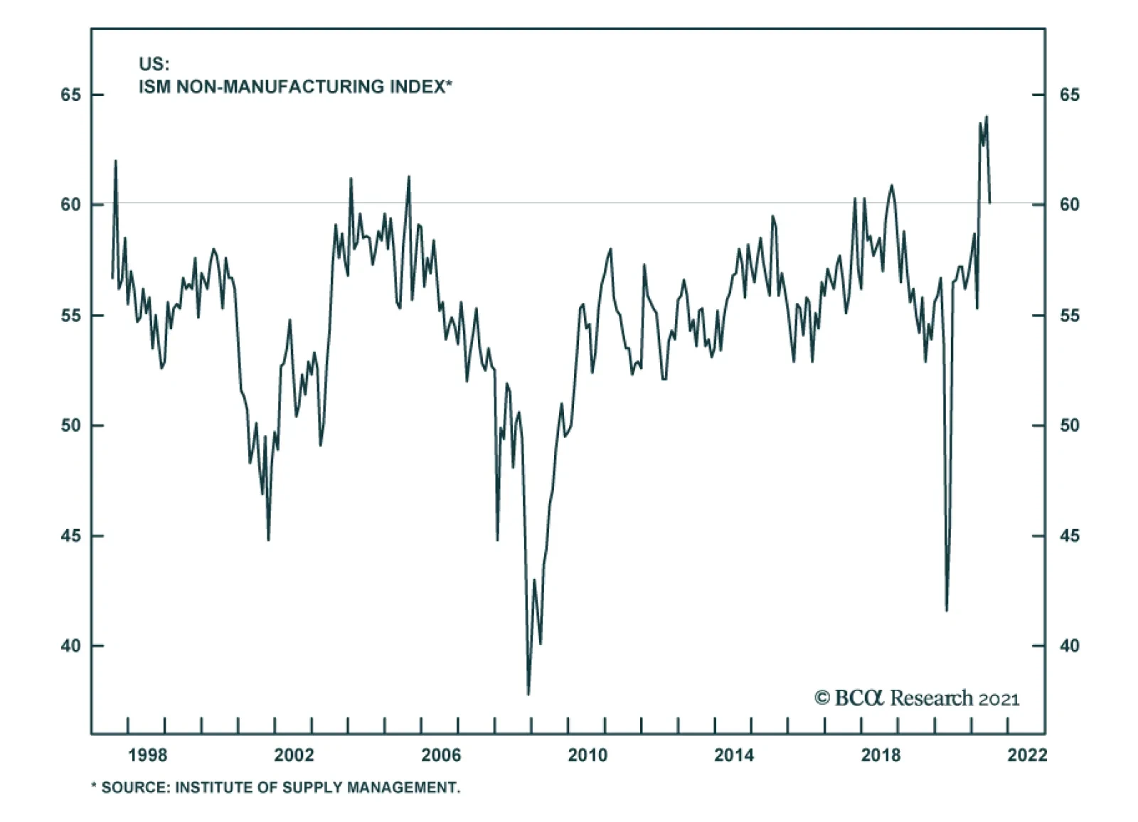
The US Services ISM reading for June fell well short of expectations on Tuesday morning, sparking a sharp Treasury rally. The 60.1 reading was quite high in level terms, suggesting that the economy is still growing robustly, but it slipped nearly four points…
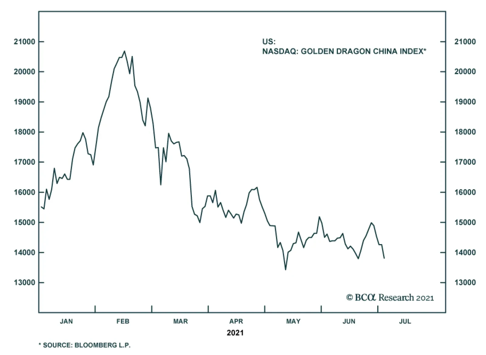
Chinese regulators asserted their authority over homegrown ride-hailing success story Didi (ticker: DIDI) by squeezing its ability to reach new customers days after it raised $4.4 billion in an IPO of American Depository Receipts (ADRs). The stock lost 20-25%…